# Variational inference and model checking

Phase 11: Probabilistic modeling · about 125 minutes · CPU

## What you will be able to do

- Derive the diagonal Gaussian variational optimum for a correlated target
- Separate optimization error from variational-family error
- Use reparameterization to inspect a Monte Carlo objective
- Diagnose mean-function mismatch using predictive residuals

## The problem

A variational optimizer finishes with a stable objective, and its posterior mean agrees with a reference. Can its uncertainty still be wrong? We will optimize a diagonal Gaussian against a correlated exact target, then check a prediction under a deliberately misspecified observation model. These are two different failure sources: an inference approximation and a model assumption.

## The idea

Variational inference fits a tractable approximation to a posterior. The approximation family limits what dependencies it can represent. A good mean estimate can coexist with a poor uncertainty estimate.

## Missing covariance can hide uncertainty

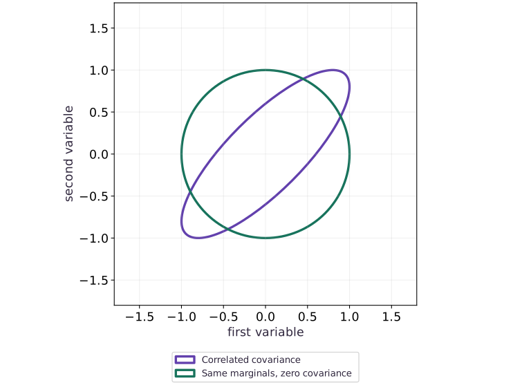
Consider two variables, each with variance $1$, and covariance $0.8$. Their sum has variance $1+1+2(0.8)=3.6$. A diagonal approximation with the same marginal variances but zero covariance would give variance $2$ for the sum.

This isolates the effect of ignoring covariance; an actual fitted approximation can also change the marginal variances. Draw covariance ellipses from the real matrices rather than sketching arbitrary shapes.

The lesson's variance comparison asks which downstream quantities are sensitive to the approximation. Check projections such as sums and differences, not only coordinate means. A different approximation family or objective can behave differently, so avoid treating one fixture as a universal direction of error.

### The covariance changes uncertainty in a sum

**Predict:** Can matching each coordinate's mean prove a correct distribution for their sum?

![The covariance changes uncertainty in a sum](../figures/probability-04-mechanism.svg)

*Architecture and dataflow mechanism diagram.*

Both analytic matrices have unit marginal variances. Purple adds covariance $0.8$, stretching along the shared diagonal; green has zero covariance. These are unit Mahalanobis-distance contours, not 95% regions or fitted samples. Sum variances are $3.6$ and $2$, respectively.

### Pause and reason

Can matching each coordinate's mean prove a correct distribution for their sum?

<details><summary>Compare your reasoning</summary>

No. The sum depends on variances and covariances too. Compare the relevant projected distribution or moments.

</details>

## Name the approximation and the KL direction

The target covariance has unit marginal variances and correlation $0.8$. Our variational family has a location $a$ and diagonal covariance $D$. It cannot tilt its uncertainty ellipse. The KL direction matters: minimizing $\operatorname{KL}(q\Vert p)$ penalizes placing probability where the target density is low. For this Gaussian target, optimizing over diagonal $D$ gives $a=m$ and $D_{ii}=1/P_{ii}$, where $P=\Sigma^{-1}$. Those are conditional-variance quantities, not the target marginal variances.

$$
\operatorname{KL}(q\Vert p)=\frac12\left[\operatorname{tr}(PD)+(a-m)^\top P(a-m)-d+\log|\Sigma|-\log|D|\right]
$$

## Work through the remaining error

For correlation $0.8$, the covariance determinant is $1-0.8^2=0.36$, and each diagonal precision is $1/0.36$. The optimal diagonal variance is therefore $0.36$. Each standard deviation is $0.6$, whereas the target marginal standard deviations are $1$. The means can be right while uncertainty is too narrow. At this optimum the KL is about $0.5108$, not zero. More optimization cannot remove that family restriction.

## Connect the exact objective to an ELBO

In a model with data $y$ and latent parameters $w$, the ELBO is the expectation of $\log p(y,w)-\log q(w)$ under $q$. The gap to log evidence is $\operatorname{KL}(q\Vert p(w\mid y))$. Reparameterize a diagonal normal as $w=a+\exp(s)\odot\epsilon$, with standard-normal $\epsilon$, to differentiate an estimated objective with respect to $a,s$. Our exact objective avoids Monte Carlo noise so the family restriction is clear. The experiment below estimates the same KL with independent random draws and compares it to the analytic value.

$$
\log p(y)-\operatorname{ELBO}(q)=\operatorname{KL}(q(w)\Vert p(w\mid y))
$$

## Inspect what the model predicts, not only its optimizer

A posterior predictive check draws plausible replicated observations and compares meaningful features with the observed data. Choose a discrepancy such as residual curvature, outlier count or group-specific spread; a single global mean can conceal a failure. Our stress fixture uses a zero linear mean and noise standard deviation $0.25$, then supplies targets $x^2-1$. Positive residuals at both ends and negative residuals near the center reveal curvature missing from the mean model. Narrower intervals cannot repair that pattern.

## Keep inference and model errors separate

The first experiment has a correct known target but an inadequate variational family. The second deliberately changes the data-generating mean while retaining an inadequate likelihood. Posterior predictive checks can reveal tension but are verified separately from model truth. For a real workflow, choose checks before inspecting a final held-out split, keep group sizes and uncertainty in reported coverage, and refit only on permitted data. **TODO (NumPyro Extension):** Compare this hand-written ELBO loop against `numpyro.infer.SVI` and `numpyro.infer.NUTS` on the same target density.

## 1. Specify a correlated target and a simpler approximation

Create a fresh main.py. Our target is an exactly known Gaussian so approximation error can be measured independently of optimization error.

```python
# Step 1 — 1. Specify a correlated target and a simpler approximation: KL here means KL(q || p).
import numpy as np
import jax
import jax.numpy as jnp
mu=jnp.array([1.,-1.])
Sigma=jnp.array([[1.,.8],[.8,1.]])
P=jnp.linalg.solve(Sigma,jnp.eye(2))
def kl(params):
    location,log_scale=params
    variance=jnp.exp(2*log_scale)
    delta=location-mu
    return .5*(jnp.sum(jnp.diag(P)*variance)+delta@P@delta-2+jnp.linalg.slogdet(Sigma)[1]-jnp.sum(2*log_scale))
```

KL here means KL(q || p). The full covariance of p is retained, while q has independent coordinates.

## 2. Optimize and compare to the exact variational optimum

Append a scan of gradient updates. The analytic optimum uses inverse diagonal precision, which differs from the target marginal variances.

```python
# Step 2 — 2. Optimize and compare to the exact variational optimum: Optimization has found the best diagonal Gaussian in this KL...
# Define `update(params, _)` to evaluate the objective and its automatic derivatives:
def update(params,_):
    # Differentiate the objective to obtain `grads` via automatic differentiation.
    grads=jax.grad(kl)(params)
    # Transform every leaf of the parameter PyTree (`new`).
    new=jax.tree.map(lambda value,grad:value-.05*grad,params,grads)
    return new,kl(new)
# Run compiled structured control flow via `jax.lax` (`(params, history)`).
params,history=jax.lax.scan(update,(jnp.zeros(2),jnp.zeros(2)),None,length=600)
location,log_scale=params
variance=jnp.exp(2*log_scale)
assert jnp.allclose(location,mu,atol=1e-4)
assert jnp.allclose(variance,1/jnp.diag(P),atol=1e-5)
assert jnp.allclose(variance,jnp.array([.36,.36]),atol=1e-5)
assert kl(params)>0.4
print('VI mean:',location,'variances:',variance,'remaining KL:',float(kl(params)))
```

Optimization has found the best diagonal Gaussian in this KL direction, yet it cannot reproduce target correlation.

## 3. Check a prediction under a changed data-generating process

Append an explicit model-mismatch experiment. The fitted line predicts zero, but new synthetic targets have curvature. Standardized residuals expose the missing structure.

```python
# Step 3 — 3. Check a prediction under a changed data-generating process: This is a deterministic stress fixture with nine targets, not an...
x=jnp.linspace(-2,2,9)
linear_mean=jnp.zeros_like(x)
noise_scale=.25
curved_targets=x**2-1.
standardized_residual=(curved_targets-linear_mean)/noise_scale
# Aggregate array values to compute `coverage`.
coverage=jnp.mean(jnp.abs(standardized_residual)<=1.96)
assert coverage<.4
assert standardized_residual[0]>10
print('synthetic nominal-95% interval coverage:',float(coverage))
print('standardized residuals:',standardized_residual)
```

This is a deterministic stress fixture with nine targets, not an estimate of population coverage. It isolates a mean-function mismatch that more posterior draws cannot repair.

## Run the example

```python
# Step 1 — 1. Specify a correlated target and a simpler approximation: KL here means KL(q || p).
import numpy as np
import jax
import jax.numpy as jnp
mu=jnp.array([1.,-1.])
Sigma=jnp.array([[1.,.8],[.8,1.]])
P=jnp.linalg.solve(Sigma,jnp.eye(2))
def kl(params):
    location,log_scale=params
    variance=jnp.exp(2*log_scale)
    delta=location-mu
    return .5*(jnp.sum(jnp.diag(P)*variance)+delta@P@delta-2+jnp.linalg.slogdet(Sigma)[1]-jnp.sum(2*log_scale))

# Step 2 — 2. Optimize and compare to the exact variational optimum: Optimization has found the best diagonal Gaussian in this KL...
# Define `update(params, _)` to evaluate the objective and its automatic derivatives:
def update(params,_):
    # Differentiate the objective to obtain `grads` via automatic differentiation.
    grads=jax.grad(kl)(params)
    # Transform every leaf of the parameter PyTree (`new`).
    new=jax.tree.map(lambda value,grad:value-.05*grad,params,grads)
    return new,kl(new)
# Run compiled structured control flow via `jax.lax` (`(params, history)`).
params,history=jax.lax.scan(update,(jnp.zeros(2),jnp.zeros(2)),None,length=600)
location,log_scale=params
variance=jnp.exp(2*log_scale)
assert jnp.allclose(location,mu,atol=1e-4)
assert jnp.allclose(variance,1/jnp.diag(P),atol=1e-5)
assert jnp.allclose(variance,jnp.array([.36,.36]),atol=1e-5)
assert kl(params)>0.4
print('VI mean:',location,'variances:',variance,'remaining KL:',float(kl(params)))

# Step 3 — 3. Check a prediction under a changed data-generating process: This is a deterministic stress fixture with nine targets, not an...
x=jnp.linspace(-2,2,9)
linear_mean=jnp.zeros_like(x)
noise_scale=.25
curved_targets=x**2-1.
standardized_residual=(curved_targets-linear_mean)/noise_scale
# Aggregate array values to compute `coverage`.
coverage=jnp.mean(jnp.abs(standardized_residual)<=1.96)
assert coverage<.4
assert standardized_residual[0]>10
print('synthetic nominal-95% interval coverage:',float(coverage))
print('standardized residuals:',standardized_residual)
```

Expected: The optimized variances are $(0.36,0.36)$, compared with target marginal variances $(1,1)$. Remaining KL is approximately $0.5108$. The curved stress fixture has visibly structured residuals and low nominal interval coverage.

## An accurate mean can coexist with underestimated uncertainty

**Predict:** Will optimizing a diagonal approximation recover the full target marginal variances?

![An accurate mean can coexist with underestimated uncertainty](../figures/probability-04.svg)

**Recorded CPU computation**

### Read the figure

The horizontal categories identify three quantities: variance of the first weight, variance of the second weight and variance of their sum. The vertical axis is variance in squared parameter units. The target bars are $1,1,3.6$. The optimized diagonal approximation gives $0.36,0.36,0.72$. The especially large gap for the sum comes from both smaller marginal variances and missing positive covariance.

### Connect it to the computation

The code checks that the optimizer reaches the analytic variational optimum. The remaining gap therefore comes from the chosen diagonal family and KL direction on this particular Gaussian target. It is not evidence that every variational approximation has the same bias; a full-covariance Gaussian can represent this target.

```python
# Compute figure data for: An accurate mean can coexist with underestimated uncertainty
visual_data={"kind":"bar","x":[0,1,2],"labels":["weight 1","weight 2","sum of weights"],"xlabel":"quantity","ylabel":"variance (squared parameter units)","series":[{"label":"exact target","y":[1.,1.,3.6]},{"label":"optimized diagonal q","y":[float(variance[0]),float(variance[1]),float(variance.sum())]}]}
```

## Recorded reference execution

CPU run: 2026-10-20T10:48:56.444623+00:00. JAX 0.9.2.

```text
VI mean: [ 0.99999994 -0.99999994] variances: [0.36000016 0.36000016] remaining KL: 0.5108256340026855
synthetic nominal-95% interval coverage: 0.2222222238779068
standardized residuals: [12.  5.  0. -3. -4. -3.  0.  5. 12.]
VI mean: [ 0.99999994 -0.99999994] variances: [0.36000016 0.36000016] remaining KL: 0.5108256340026855
synthetic nominal-95% interval coverage: 0.2222222238779068
standardized residuals: [12.  5.  0. -3. -4. -3.  0.  5. 12.]
Monte Carlo KL: 0.5119153261184692
model self-coverage: 0.9493999481201172
PASS: probability-04

```

## Monte Carlo KL through reparameterization

**Predict before running:** Will an estimate from diagonal-normal draws approach the exact KL even though the approximation is imperfect?

```python
# Experiment — Monte Carlo KL through reparameterization: Matching the exact KL validates this estimator on the fixture;...
# Create or split explicit PRNG key(s) (`eps`) for reproducible randomness.
eps=jax.random.normal(jax.random.key(52),(40000,2))
z=location+jnp.exp(log_scale)*eps
delta=z-mu
logp=-.5*(jnp.einsum('ni,ij,nj->n',delta,P,delta)+2*jnp.log(2*jnp.pi)+jnp.linalg.slogdet(Sigma)[1])
# Reduce along axis=1 to compute `logq`.
logq=-.5*jnp.sum(eps**2,axis=1)-jnp.sum(log_scale)-jnp.log(2*jnp.pi)
# Aggregate array values to compute `estimate`.
estimate=jnp.mean(logq-logp)
assert abs(float(estimate-kl(params)))<.03
print('Monte Carlo KL:',float(estimate))
```

**Expected:** The estimate is close to the exact nonzero KL of $0.5108$.

Matching the exact KL validates this estimator on the fixture; it does not imply the approximate posterior is exact.

## Count model-generated intervals

**Predict before running:** Under the stated zero-mean normal model, what fraction of many replicated observations lies within 1.96 noise scales?

```python
# Experiment — Count model-generated intervals: Self-coverage checks interval arithmetic under the model.
# Create or split explicit PRNG key(s) (`replicated`) for reproducible randomness.
replicated=.25*jax.random.normal(jax.random.key(83),(40000,))
# Aggregate array values to compute `model_coverage`.
model_coverage=jnp.mean(jnp.abs(replicated)<=1.96*.25)
assert .94<model_coverage<.96
print("model self-coverage:",float(model_coverage))
```

**Expected:** Approximately $95\%$ lie inside their model interval.

Self-coverage checks interval arithmetic under the model. It is distinct from coverage under the curved alternative.

## Make it yours

Replace the target correlation by zero and rederive the optimal diagonal variances and minimum KL. Verify that the diagonal family can now represent the target exactly.

### How to write this exercise — Step-by-step recipe & starter scaffold

**Key functions & syntax to use:**
- `jnp.zeros / jnp.ones(shape, dtype=...)` — Allocates a tensor of the given `shape` initialized with constants.
- `x.sum(axis=...) / x.mean(axis=..., keepdims=...)` — Reduces values along the named `axis` (the axis you name is collapsed unless `keepdims=True`).
- `jnp.allclose(actual, expected, rtol=..., atol=...)` — Checks that two arrays match elementwise within floating-point tolerance.

**Step-by-step implementation plan:**
1. Set up the changed input or configuration parameters requested in the prompt.
2. Run the target function or transformation and assert that the output matches your prediction.

**Starter code scaffold (fill in the TODOs):**

```python
# Exercise solution: Replace the target correlation by zero and rederive the optimal...
def independent_kl(location,log_scale):
    return ...  # TODO: return computed result
assert jnp.allclose(independent_kl(mu,jnp.zeros(2)),0.)  # TODO: complete assertion check
```

<details><summary>Reference solution</summary>

```python
# Exercise solution: Replace the target correlation by zero and rederive the optimal...
def independent_kl(location,log_scale):
    return .5*(jnp.sum(jnp.exp(2*log_scale))+jnp.sum((location-mu)**2)-2-jnp.sum(2*log_scale))
assert jnp.allclose(independent_kl(mu,jnp.zeros(2)),0.)
```

</details>

## A correct diagonal is not a correct covariance

**Transfer / diagnosis**

Compare the variance of the sum of two target coordinates with that under the optimized diagonal approximation.

<details><summary>Hint</summary>

Retain the off-diagonal covariance terms in the target calculation.

</details>

### How to write: A correct diagonal is not a correct covariance — Step-by-step recipe & starter scaffold

**Key functions & syntax to use:**
- `jnp.zeros / jnp.ones(shape, dtype=...)` — Allocates a tensor of the given `shape` initialized with constants.
- `x.sum(axis=...) / x.mean(axis=..., keepdims=...)` — Reduces values along the named `axis` (the axis you name is collapsed unless `keepdims=True`).
- `jnp.allclose(actual, expected, rtol=..., atol=...)` — Checks that two arrays match elementwise within floating-point tolerance.

**Step-by-step implementation plan:**
1. Perform matrix / vector contraction (`@`) to compute `true_sum_var`.
2. Aggregate array values to compute `approx_sum_var`.

**Starter code scaffold (fill in the TODOs):**

```python
# A correct diagonal is not a correct covariance (Transfer / diagnosis): Joint predictions can reveal approximation error that...
direction = jnp.ones(...)  # TODO: compute direction
# Perform matrix / vector contraction (`@`) to compute `true_sum_var`.
true_sum_var = ...  # TODO: compute true_sum_var
# Aggregate array values to compute `approx_sum_var`.
approx_sum_var = jnp.sum(...)  # TODO: compute approx_sum_var
assert jnp.allclose(true_sum_var,3.6)  # TODO: complete assertion check
assert jnp.allclose(approx_sum_var,.72,atol=1e-5)  # TODO: complete assertion check
```

<details><summary>Reference solution and reasoning</summary>

```python
# A correct diagonal is not a correct covariance (Transfer / diagnosis): Joint predictions can reveal approximation error that...
direction=jnp.ones(2)
# Perform matrix / vector contraction (`@`) to compute `true_sum_var`.
true_sum_var=direction@Sigma@direction
# Aggregate array values to compute `approx_sum_var`.
approx_sum_var=jnp.sum(variance)
assert jnp.allclose(true_sum_var,3.6)
assert jnp.allclose(approx_sum_var,.72,atol=1e-5)
```

Joint predictions can reveal approximation error that examining means alone completely misses.

</details>

## Repair the changed mean without hiding noise

**Transfer / diagnosis**

Replace the zero mean by the known curved mean in the stress fixture. Draw fresh noisy targets and compare residual spread to the stated noise scale.

<details><summary>Hint</summary>

The fixture supplies the true curvature; real data would require fitting and held-out evaluation.

</details>

### How to write: Repair the changed mean without hiding noise — Step-by-step recipe & starter scaffold

**Key functions & syntax to use:**
- `jnp.linspace(start, stop, num)` — Creates `num` evenly spaced float points across the closed interval `[start, stop]`.
- `x.sum(axis=...) / x.mean(axis=..., keepdims=...)` — Reduces values along the named `axis` (the axis you name is collapsed unless `keepdims=True`).
- `jax.random.PRNGKey(seed) & jax.random.split(key)` — Manages explicit, stateless PRNG keys—always split a key before passing subkeys into independent random draws.

**Step-by-step implementation plan:**
1. Create or split explicit PRNG key(s) (`fresh`) for reproducible randomness.

**Starter code scaffold (fill in the TODOs):**

```python
# Repair the changed mean without hiding noise (Transfer / diagnosis): Correcting the mean removes systematic residual structure in...
truth = jnp.linspace(...)  # TODO: compute truth
# Create or split explicit PRNG key(s) (`fresh`) for reproducible randomness.
fresh = ...  # TODO: compute fresh
residual = ...  # TODO: compute residual
assert abs(float(residual.std())-.25)  # TODO: complete assertion check
assert abs(float(residual.mean()))  # TODO: complete assertion check
```

<details><summary>Reference solution and reasoning</summary>

```python
# Repair the changed mean without hiding noise (Transfer / diagnosis): Correcting the mean removes systematic residual structure in...
truth=jnp.linspace(-2,2,20000)**2-1
# Create or split explicit PRNG key(s) (`fresh`) for reproducible randomness.
fresh=truth+.25*jax.random.normal(jax.random.key(95),(20000,))
residual=fresh-truth
assert abs(float(residual.std())-.25)<.01
assert abs(float(residual.mean()))<.01
```

Correcting the mean removes systematic residual structure in this known simulation; observation noise remains.

</details>

## Check your understanding

The variational mean is correct and the optimization gradient is tiny. Why can posterior intervals still be too narrow?

1. The diagonal family cannot represent the correlated target, even at its optimum
2. Any Gaussian model necessarily produces wrong uncertainty
3. The number of optimizer iterations defines posterior variance

<details><summary>Answer and explanation</summary>

The diagonal family cannot represent the correlated target, even at its optimum

For this KL direction and correlated target, the optimal diagonal variances are 0.36 rather than the target marginal variances of one. This is approximation error, not an unfinished optimizer.

</details>

## Diagnose the result

If the objective has stopped improving, compare to the independent analytic optimum before adding iterations. If parameter uncertainty looks plausible but residuals show a U-shaped trend, investigate the mean model. If only one group is poorly covered, keep group-specific checks instead of relying on aggregate coverage.

## Carry forward

- An optimized approximation can still miss posterior covariance.
- Model self-coverage is weaker than evaluation under changed observations.
- Keep inference diagnostics and posterior predictive checks as separate evidence.

## Keep your evidence

Analytic and optimized KL, variance comparison, Monte Carlo estimate and explained residual stress fixture. Keep the environment, observed outputs and your explanation of the figure.

Save your predictions, modified code, terminal outputs, and reasoning in your engineering portfolio.

## Primary references

- [Stan variational inference](https://mc-stan.org/docs/reference-manual/variational.html)
- [Stan posterior predictive checks](https://mc-stan.org/docs/stan-users-guide/posterior-predictive-checks.html)
- [NumPyro SVI interface](https://num.pyro.ai/en/stable/svi.html)