# Vectorize trajectories and scan time

Phase 10: Scientific computing · about 100 minutes · CPU

## What you will be able to do

- Construct and verify a fourth-order fixed-step transition.
- Distinguish batch-major from time-major trajectory layouts.
- Compare two valid scan/vectorization compositions numerically.
- Separate independent ensembles from interacting states.

## The problem

You need to simulate a collection of experimental starts, not just one. Which dimension represents independent experiments, and which represents sequential time? We will build both compositions explicitly and verify that their axes and physical predictions agree.

## The idea

A simulation ensemble repeats one rule across independent systems and across time. Vectorization handles the independent systems; recurrence handles each system's evolving state. Name those axes before composing transforms.

## There are two different axes of repetition

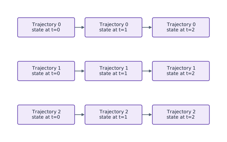
Picture a grid with time running left to right and one independent trajectory per row. State arrows connect adjacent times within a row. No state arrow crosses into another trajectory unless the physical model explicitly couples them.

Initial conditions can vary by trajectory while a physical parameter stays shared, or both may vary. That is an argument-mapping choice, not merely a shape convenience. Record it before applying vectorization.

The trajectory plot shows outputs of that grid. Preserve the returned time/batch axis order when plotting; an accidental transpose can connect different systems instead of successive times. Compare one row with an independently run single trajectory.

### Vectorize across systems; scan through time

**Predict:** What should happen if you permute independent initial conditions?

![Vectorize across systems; scan through time](../figures/science-02-mechanism.svg)

*Architecture and dataflow mechanism diagram.*

Each row is an independent initial condition. Horizontal arrows advance only that system; there are no cross-row state dependencies. Vectorization groups rows and scan represents recurrence. Boxes show state positions in the computation, not physical coordinates or measured durations.

### Pause and reason

What should happen if you permute independent initial conditions?

<details><summary>Compare your reasoning</summary>

The trajectories should undergo the same permutation, with each trajectory's time evolution unchanged. This checks independence and axis handling.

</details>

## Improve one step before multiplying trajectories

Forward Euler samples the slope only at the start of the interval. Classical RK4 samples a start slope, two midpoint slopes and an endpoint slope, then combines them with weights $1,2,2,1$. The intermediate states are trial values, not four extra saved observations. For our linear equation the full step is multiplication by a fourth-degree approximation to $e^{-kh}$. This makes an independent algebraic oracle possible.

$$
R(z)=1+z+\frac{z^2}{2}+\frac{z^3}{6}+\frac{z^4}{24},\qquad u_{n+1}=R(-kh)u_n
$$

## Read shapes as physical statements

Three initial values and forty updates produce a batch-major array of shape $(3,41)$. Row $b$ is one trajectory; column $n$ holds all experiment values at time $nh$. The extra time point is the initial state. We deliberately use different axis sizes to make an accidental transpose visible. A mean over the batch answers a different question from a mean over time.

## One transformation handles independence; another handles dependency

vmap transforms a scalar simulation into an ensemble operation. scan still enforces the sequential state dependence inside each trajectory. Reversing the composition is possible here: the carry can hold all three independent states, giving a time-major result of shape $(41,3)$. Its transpose matches the first construction. If one trajectory exchanges heat with another, the batch members no longer obey independent scalar equations; write a coupled vector state instead.

## Use physical structure as a second check

This equation is linear in the initial state. Starting at $2$ must produce four times the trajectory starting at $0.5$. That check is separate from the exponential comparison and catches unintended normalization over the batch axis. Linearity is special to this model; do not impose it on a nonlinear reaction model simply because batching worked here.

## Choose saved outputs deliberately

Saving every state costs storage proportional to batch size times number of saved times. Some objectives need only the final state. In that case return no saved observation from scan and keep its final carry. This reduces the explicit output size; it does not by itself establish the memory cost of reverse-mode differentiation, which may retain or recompute intermediates.

## Use a higher-order scalar transition

Append this block to main.py in your CPU course environment; for the first block create the file. Run blocks in order.

```python
# Step 1 — Use a higher-order scalar transition: Runge–Kutta uses four slopes inside one step.
import jax
# Update state in place with the new values.
jax.config.update("jax_enable_x64", True)
import jax.numpy as jnp
import numpy as np

def rk4_step(rate, value, dt):
    a = -rate*value
    b = -rate*(value + dt*a/2)
    c = -rate*(value + dt*b/2)
    d = -rate*(value + dt*c)
    return value + dt*(a + 2*b + 2*c + d)/6

# Define `solve(rate, initial, steps, dt)` to carry state across steps with `jax.lax.scan`:
def solve(rate, initial, steps=40, dt=0.05):
    def advance(value, unused):
        next_value = rk4_step(rate, value, dt)
        return next_value, next_value
    # Run compiled structured control flow via `jax.lax` (`(_, tail)`).
    _, tail = jax.lax.scan(advance, initial, None, length=steps)
    return jnp.concatenate((jnp.atleast_1d(initial), tail))
```

Runge–Kutta uses four slopes inside one step. It remains a pure transition, so the same scan interface can save its trajectory.

## Batch initial conditions while sharing the model

Append this block to main.py in your CPU course environment; for the first block create the file. Run blocks in order.

```python
# Step 2 — Batch initial conditions while sharing the model: The batch axis is independent initial conditions, not time.
initials = jnp.array([0.5, 1.0, 2.0])
rate, dt, steps = 0.7, 0.05, 40
# Vectorize across the batch dimension with `jax.vmap` (`simulate_batch`).
simulate_batch = jax.jit(jax.vmap(lambda initial: solve(rate, initial, steps, dt)))
trajectories = simulate_batch(initials)
times = np.arange(steps+1)*dt
# Convert `oracle` to a host NumPy array for inspection or verification.
oracle = np.asarray(initials)[:,None]*np.exp(-rate*times[None,:])
# Check tensor shape invariant: `trajectories.shape == (3, 41)`
assert trajectories.shape == (3, 41)
np.testing.assert_allclose(trajectories, oracle, rtol=3e-8, atol=1e-10)
# Convert `` to a host NumPy array for inspection or verification.
np.testing.assert_allclose(np.asarray(trajectories)[2], 4*np.asarray(trajectories)[0], rtol=1e-12)
print("Shape:", trajectories.shape, "endpoints:", np.asarray(trajectories)[:,-1])
```

The batch axis is independent initial conditions, not time. The shared rate and grid are closed over here; vmap adds one leading axis to the scalar solve.

## Change composition and verify axis meaning

Append this block to main.py in your CPU course environment; for the first block create the file. Run blocks in order.

```python
# Step 3 — Change composition and verify axis meaning: Array arithmetic applies the independent scalar dynamics to all...
# Define `scan_batch(rate, values, steps, dt)` to carry state across steps with `jax.lax.scan`:
def scan_batch(rate, values, steps=40, dt=0.05):
    def advance(state, unused):
        updated = rk4_step(rate, state, dt)
        return updated, updated
    # Run compiled structured control flow via `jax.lax` (`(_, tail)`).
    _, tail = jax.lax.scan(advance, values, None, length=steps)
    return jnp.concatenate((values[None,:], tail), axis=0)
# Run compiled structured control flow via `jax.lax` (`time_major`).
time_major = scan_batch(rate, initials)
# Check tensor shape invariant: `time_major.shape == (41, 3)`
assert time_major.shape == (41, 3)
np.testing.assert_allclose(time_major.T, trajectories, rtol=1e-12, atol=1e-12)
print("scan(vectors) transposed equals vmap(scan)")
```

Array arithmetic applies the independent scalar dynamics to all initial conditions. This equivalence would fail if the model coupled different batch members.

## Run the example

```python
# Step 1 — Use a higher-order scalar transition: Runge–Kutta uses four slopes inside one step.
import jax
# Update state in place with the new values.
jax.config.update("jax_enable_x64", True)
import jax.numpy as jnp
import numpy as np

def rk4_step(rate, value, dt):
    a = -rate*value
    b = -rate*(value + dt*a/2)
    c = -rate*(value + dt*b/2)
    d = -rate*(value + dt*c)
    return value + dt*(a + 2*b + 2*c + d)/6

# Define `solve(rate, initial, steps, dt)` to carry state across steps with `jax.lax.scan`:
def solve(rate, initial, steps=40, dt=0.05):
    def advance(value, unused):
        next_value = rk4_step(rate, value, dt)
        return next_value, next_value
    # Run compiled structured control flow via `jax.lax` (`(_, tail)`).
    _, tail = jax.lax.scan(advance, initial, None, length=steps)
    return jnp.concatenate((jnp.atleast_1d(initial), tail))

# Step 2 — Batch initial conditions while sharing the model: The batch axis is independent initial conditions, not time.
initials = jnp.array([0.5, 1.0, 2.0])
rate, dt, steps = 0.7, 0.05, 40
# Vectorize across the batch dimension with `jax.vmap` (`simulate_batch`).
simulate_batch = jax.jit(jax.vmap(lambda initial: solve(rate, initial, steps, dt)))
trajectories = simulate_batch(initials)
times = np.arange(steps+1)*dt
# Convert `oracle` to a host NumPy array for inspection or verification.
oracle = np.asarray(initials)[:,None]*np.exp(-rate*times[None,:])
# Check tensor shape invariant: `trajectories.shape == (3, 41)`
assert trajectories.shape == (3, 41)
np.testing.assert_allclose(trajectories, oracle, rtol=3e-8, atol=1e-10)
# Convert `` to a host NumPy array for inspection or verification.
np.testing.assert_allclose(np.asarray(trajectories)[2], 4*np.asarray(trajectories)[0], rtol=1e-12)
print("Shape:", trajectories.shape, "endpoints:", np.asarray(trajectories)[:,-1])

# Step 3 — Change composition and verify axis meaning: Array arithmetic applies the independent scalar dynamics to all...
# Define `scan_batch(rate, values, steps, dt)` to carry state across steps with `jax.lax.scan`:
def scan_batch(rate, values, steps=40, dt=0.05):
    def advance(state, unused):
        updated = rk4_step(rate, state, dt)
        return updated, updated
    # Run compiled structured control flow via `jax.lax` (`(_, tail)`).
    _, tail = jax.lax.scan(advance, values, None, length=steps)
    return jnp.concatenate((values[None,:], tail), axis=0)
# Run compiled structured control flow via `jax.lax` (`time_major`).
time_major = scan_batch(rate, initials)
# Check tensor shape invariant: `time_major.shape == (41, 3)`
assert time_major.shape == (41, 3)
np.testing.assert_allclose(time_major.T, trajectories, rtol=1e-12, atol=1e-12)
print("scan(vectors) transposed equals vmap(scan)")
```

Expected: Shape (3, 41); endpoints approximately [0.12329849, 0.24659697, 0.49319394]. Both compositions agree.

## Batching preserves independent physical trajectories

**Predict:** Should the highest curve decay proportionally faster, or preserve its ratio to the other curves?

![Batching preserves independent physical trajectories](../figures/science-02.svg)

**Recorded CPU computation**

### Read the figure

Time in seconds runs horizontally; excess temperature runs vertically. The three curves correspond to initial values $0.5$, $1$ and $2$. Each is one row of the batch-major output, including its initial observation.

At two seconds their values are approximately $0.1233$, $0.2466$ and $0.4932$. Their absolute changes differ, but every curve retains the same fraction of its initial value. The highest remains four times the lowest throughout.

### Connect it to the computation

The common rate produces that shared relative decay. vmap adds independent experiments without inserting a mean, normalization or interaction between them. The code checks both this proportional relationship and the analytic exponential.

The plot has no runtime or memory axis. It establishes numerical behavior for this ensemble, not a speedup from vectorization. The last lesson adds synchronized measurements with their own limitations.

```python
# Compute figure data for: Batching preserves independent physical trajectories
# Convert `visual_data` to a host NumPy array for inspection or verification.
visual_data={'kind':'line','x':times.tolist(),'xlabel':'time (seconds)','ylabel':'excess temperature','series':[{'label':f'initial {float(u):g}','y':np.asarray(trajectories)[i].tolist()} for i,u in enumerate(initials)]}
```

## Recorded reference execution

CPU run: 2026-10-20T10:47:57.386723+00:00. JAX 0.9.2.

```text
Shape: (3, 41) endpoints: [0.12329848 0.24659697 0.49319394]
scan(vectors) transposed equals vmap(scan)
Shape: (3, 41) endpoints: [0.12329848 0.24659697 0.49319394]
scan(vectors) transposed equals vmap(scan)
RK4 polynomial maximum difference: 1.4432899320127035e-15
Paired-rate endpoints: [0.33516002 0.24659697 0.22160636]
Permutation preserves trajectory identity
Only final states returned: [0.12329848 0.24659697 0.49319394]
Grid axes: rate, initial condition, time (3, 3, 41)
PASS: science-02

```

## Compare RK4 with an independent polynomial

**Predict before running:** If the step is correct, can a loop-free formula reproduce every saved state?

```python
# Experiment — Compare RK4 with an independent polynomial: This checks the discrete algorithm independently of the...
z = -rate*dt
multiplier = 1 + z + z*z/2 + z**3/6 + z**4/24
polynomial = np.asarray(initials)[:,None]*multiplier**np.arange(steps+1)[None,:]
np.testing.assert_allclose(trajectories, polynomial, rtol=1e-12, atol=1e-12)
print("RK4 polynomial maximum difference:", np.max(np.abs(np.asarray(trajectories)-polynomial)))
```

**Expected:** Differences are near float64 roundoff.

This checks the discrete algorithm independently of the continuous exponential. RK4 has much smaller error here but is not exact.

## Let each trajectory have its own rate

**Predict before running:** Which argument axes should map if rates and initial conditions are paired?

```python
# Experiment — Let each trajectory have its own rate: Mapping both axes pairs corresponding entries.
rates = jnp.array([0.2, 0.7, 1.1])
# Vectorize across the batch dimension with `jax.vmap` (`paired`).
paired = jax.vmap(lambda k, u: solve(k,u), in_axes=(0,0))(rates,initials)
# Convert `paired_reference` to a host NumPy array for inspection or verification.
paired_reference = np.asarray(initials)[:,None]*np.exp(-np.asarray(rates)[:,None]*times)
np.testing.assert_allclose(paired,paired_reference,rtol=2e-7,atol=1e-10)
print("Paired-rate endpoints:", np.asarray(paired)[:,-1])
```

**Expected:** Three trajectories now have different relative decay rates.

Mapping both axes pairs corresponding entries. A grid of every rate with every initial value would require nested mapping and a different output contract.

## Make it yours

Add a fourth initial condition, verify the changed output shape and exponential values, then verify that reordering initial conditions reorders rows only.

### How to write this exercise — Step-by-step recipe & starter scaffold

**Key functions & syntax to use:**
- `jnp.array(values, dtype=...)` — Constructs an immutable device-backed JAX array from Python/NumPy values.
- `jnp.allclose(actual, expected, rtol=..., atol=...)` — Checks that two arrays match elementwise within floating-point tolerance.
- `jax.vmap(fn, in_axes=..., out_axes=...)` — Vectorizes a single-example function across a batch axis without writing a Python loop.

**Step-by-step implementation plan:**
1. Vectorize across the batch dimension with `jax.vmap` (`changed`).
2. Check tensor shape invariant: `changed.shape == (4,41)`
3. Convert `` to a host NumPy array for inspection or verification.
4. Vectorize across the batch dimension with `jax.vmap` (`reordered`).

**Starter code scaffold (fill in the TODOs):**

```python
# Exercise solution: Add a fourth initial condition, verify the changed output shape and...
changed_initials = jnp.array(...)  # TODO: compute changed_initials
# Vectorize across the batch dimension with `jax.vmap` (`changed`).
changed = jax.vmap(...)  # TODO: compute changed
# Check tensor shape invariant: `changed.shape == (4,41)`
assert changed.shape  # TODO: complete assertion check
# Convert `` to a host NumPy array for inspection or verification.
np.testing.assert_allclose(changed,np.asarray(changed_initials)[:,None]*np.exp(-0.7*times),rtol=3e-8)
order = jnp.array(...)  # TODO: compute order
# Vectorize across the batch dimension with `jax.vmap` (`reordered`).
reordered = jax.vmap(...)  # TODO: compute reordered
np.testing.assert_allclose(reordered,changed[order],rtol = ...  # TODO: compute np.testing.assert_allclose(reordered,changed[order],rtol
print("Permutation preserves trajectory identity")
```

<details><summary>Reference solution</summary>

```python
# Exercise solution: Add a fourth initial condition, verify the changed output shape and...
changed_initials = jnp.array([0.5, 1.0, 2.0, 3.0])
# Vectorize across the batch dimension with `jax.vmap` (`changed`).
changed = jax.vmap(lambda u: solve(0.7,u))(changed_initials)
# Check tensor shape invariant: `changed.shape == (4,41)`
assert changed.shape == (4,41)
# Convert `` to a host NumPy array for inspection or verification.
np.testing.assert_allclose(changed,np.asarray(changed_initials)[:,None]*np.exp(-0.7*times),rtol=3e-8)
order = jnp.array([3,0,2,1])
# Vectorize across the batch dimension with `jax.vmap` (`reordered`).
reordered = jax.vmap(lambda u: solve(0.7,u))(changed_initials[order])
np.testing.assert_allclose(reordered,changed[order],rtol=1e-12)
print("Permutation preserves trajectory identity")
```

</details>

## Save only what the objective needs

**Practice**

Implement a final-state-only solve and compare it with the final column of the saved batch. Explain which allocation was removed.

<details><summary>Hint</summary>

scan may emit None while its carry still advances.

</details>

### How to write: Save only what the objective needs — Step-by-step recipe & starter scaffold

**Key functions & syntax to use:**
- `jnp.allclose(actual, expected, rtol=..., atol=...)` — Checks that two arrays match elementwise within floating-point tolerance.
- `jax.vmap(fn, in_axes=..., out_axes=...)` — Vectorizes a single-example function across a batch axis without writing a Python loop.
- `jax.lax.scan(step_fn, init_carry, xs, length=...)` — Compiles a sequential loop where `step_fn(carry, x)` returns `(next_carry, y)`, returning `(final_carry, stacked_ys)`.

**Step-by-step implementation plan:**
1. Define `final_only(rate, initial, steps, dt)` to carry state across steps with `jax.lax.scan`:
2. Vectorize across the batch dimension with `jax.vmap` (`finals`).

**Starter code scaffold (fill in the TODOs):**

```python
# Save only what the objective needs (Practice): The explicit trajectory output is removed.
# Define `final_only(rate, initial, steps, dt)` to carry state across steps with `jax.lax.scan`:
def final_only(rate, initial, steps=40, dt=0.05):
    def advance(value, unused):
        return ...  # TODO: return computed result
    return jax.lax.scan(advance,initial,None,length = ...  # TODO: compute return jax.lax.scan(advance,initial,None,length
# Vectorize across the batch dimension with `jax.vmap` (`finals`).
finals = jax.vmap(...)  # TODO: compute finals
np.testing.assert_allclose(finals,trajectories[:,-1],rtol=1e-12)
print("Only final states returned:", np.asarray(finals))
```

<details><summary>Reference solution and reasoning</summary>

```python
# Save only what the objective needs (Practice): The explicit trajectory output is removed.
# Define `final_only(rate, initial, steps, dt)` to carry state across steps with `jax.lax.scan`:
def final_only(rate, initial, steps=40, dt=0.05):
    def advance(value, unused):
        return rk4_step(rate,value,dt), None
    return jax.lax.scan(advance,initial,None,length=steps)[0]
# Vectorize across the batch dimension with `jax.vmap` (`finals`).
finals = jax.vmap(lambda u: final_only(0.7,u))(initials)
np.testing.assert_allclose(finals,trajectories[:,-1],rtol=1e-12)
print("Only final states returned:", np.asarray(finals))
```

The explicit trajectory output is removed. Differentiation memory requires separate analysis and measurement.

</details>

## Pairing versus Cartesian products

**Challenge**

Build the full grid of three rates and three initial values. Show that its diagonal agrees with the paired-rate experiment.

<details><summary>Hint</summary>

Use nested vmap; identify the rate, initial-condition and time axes explicitly.

</details>

### How to write: Pairing versus Cartesian products — Step-by-step recipe & starter scaffold

**Key functions & syntax to use:**
- `jnp.arange(n, dtype=...)` — Creates a 1-D JAX array of evenly spaced values `[0, 1, ..., n-1]` on the target device.
- `jnp.allclose(actual, expected, rtol=..., atol=...)` — Checks that two arrays match elementwise within floating-point tolerance.
- `jax.vmap(fn, in_axes=..., out_axes=...)` — Vectorizes a single-example function across a batch axis without writing a Python loop.

**Step-by-step implementation plan:**
1. Vectorize across the batch dimension with `jax.vmap` (`grid`).
2. Check tensor shape invariant: `grid.shape == (3,3,41)`
3. Create evenly spaced index values in ``.

**Starter code scaffold (fill in the TODOs):**

```python
# Pairing versus Cartesian products (Challenge): Paired batches and Cartesian products are different experiments.
# Vectorize across the batch dimension with `jax.vmap` (`grid`).
grid = jax.vmap(...)  # TODO: compute grid
# Check tensor shape invariant: `grid.shape == (3,3,41)`
assert grid.shape  # TODO: complete assertion check
# Create evenly spaced index values in ``.
np.testing.assert_allclose(grid[jnp.arange(3),jnp.arange(3)],paired,rtol = ...  # TODO: compute np.testing.assert_allclose(grid[jnp.arange(3),jnp.arange(3)],paired,rtol
print("Grid axes: rate, initial condition, time", grid.shape)
```

<details><summary>Reference solution and reasoning</summary>

```python
# Pairing versus Cartesian products (Challenge): Paired batches and Cartesian products are different experiments.
# Vectorize across the batch dimension with `jax.vmap` (`grid`).
grid = jax.vmap(lambda k: jax.vmap(lambda u: solve(k,u))(initials))(rates)
# Check tensor shape invariant: `grid.shape == (3,3,41)`
assert grid.shape == (3,3,41)
# Create evenly spaced index values in ``.
np.testing.assert_allclose(grid[jnp.arange(3),jnp.arange(3)],paired,rtol=1e-12)
print("Grid axes: rate, initial condition, time", grid.shape)
```

Paired batches and Cartesian products are different experiments. The diagonal correspondence verifies the axis interpretation.

</details>

## Check your understanding

What does a shape of (3, 41) mean in the batch-major solver?

1. Three independent initial conditions, each with the initial state plus forty updates.
2. Three time points, each with forty-one parameters.
3. Forty-one independent devices.

<details><summary>Answer and explanation</summary>

Three independent initial conditions, each with the initial state plus forty updates.

vmap contributes the leading independent-experiment axis. The scalar solve contributes its forty-one saved states; no device placement is specified.

</details>

## Diagnose the result

If the reference comparison broadcasts unexpectedly, print both shapes before reducing anything. Compare a named row and a named time column. If changing one initial condition changes other rows, inspect reductions or coupling across the batch. A reduction can hide an axis error while still producing a plausible scalar.

## Carry forward

- Improve one step before multiplying trajectories
- Read shapes as physical statements
- One transformation handles independence; another handles dependency
- Use physical structure as a second check
- Choose saved outputs deliberately

## Keep your evidence

Polynomial/exponential references, batch/time shape diagram, permutation and final-only checks. Keep the environment, observed outputs and your explanation of the figure.

Save your predictions, modified code, terminal outputs, and reasoning in your engineering portfolio.

## Primary references

- [JAX scan: fixed carry structure and reverse-mode differentiation](https://docs.jax.dev/en/latest/_autosummary/jax.lax.scan.html)
- [JAX automatic vectorization](https://docs.jax.dev/en/latest/_autosummary/jax.vmap.html)
- [JAX derivative checking and Jacobian products](https://docs.jax.dev/en/latest/notebooks/autodiff_cookbook.html)
- [Diffrax solver terms, saved values and solution inspection](https://docs.kidger.site/diffrax/usage/getting-started/)