Reversible Backprop as a custom_vjp in JAX
#integrators#reversibility#memory#jax#flax#nnx#implementation
Part 4 of 5Networks as Integrators
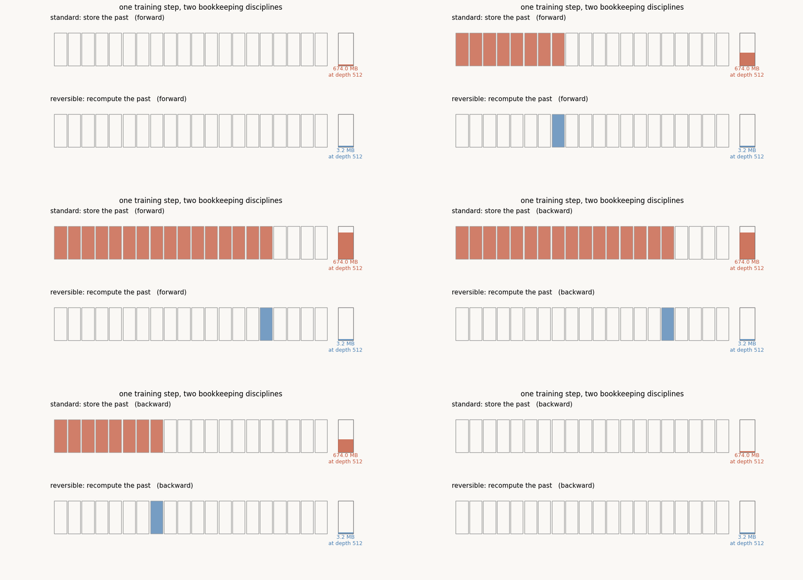
The whole memory claim rests on one tuple. The forward rule below hands back the parameters and the final state as its residuals, and nothing indexed by depth; at 512 layers that is 3.2 MB of scratch where standard backprop reserves 674. The explainer argues the case; here are the block’s exact inverse, the jax.custom_vjp that walks the trajectory backward rather than storing it, XLA’s own reading of the compiled step, and the float32 cliff reproduced in twenty lines of numpy. Code blocks are quoted from the Kaggle run (bundle kgl_blog-revmem-v1), not paraphrased.
The block and its undo
One momentum layer, and the two lines that reverse it:
def block(p, x):
    return jnp.tanh(x @ p["w1"] + p["b1"]) @ p["w2"] + p["b2"]

# forward:  v' = MU * v + block(p, x);  x' = x + H_STEP * v'
# inverse:  x  = x' - H_STEP * v';      v = (v' - block(p, x)) / MU
The inverse needs nothing but the endpoint and the same block. That is the entire storage story: if the backward pass can call these two lines, it does not need the forward pass to have banked anything.
The custom_vjp that recomputes instead of remembering
JAX lets a function declare its own backward rule. The forward rule saves only the output state as residuals, a constant amount of memory at any depth. The backward rule then reconstructs each layer’s input by inversion, and having just recovered it, backprops through that one layer with an ordinary jax.vjp, accumulating parameter gradients as it walks:
@jax.custom_vjp
def rev_forward(p, x0, v0, L_arr):
    L = L_arr.shape[0]
    return fwd_scan(p, x0, v0, L)

def rev_fwd(p, x0, v0, L_arr):
    out = rev_forward(p, x0, v0, L_arr)
    # residuals: ONLY the output state (constant in depth), never the trajectory
    return out, (p, out[0], out[1], L_arr)

def rev_bwd(res, g):
    p, xL, vL, L_arr = res
    gx, gv = g

    def back(carry, _):
        x_next, v_next, gx_n, gv_n, gp = carry
        # invert one layer to recover its input
        x_prev = x_next - H_STEP * v_next
        f_val, f_vjp = jax.vjp(lambda pp, xx: block(pp, xx), p, x_prev)
        v_prev = (v_next - f_val) / MU
        # backprop the same layer given recovered inputs
        gv_local = gv_n + H_STEP * gx_n
        gp_f, gx_f = f_vjp(gv_local)
        gx_p = gx_n + gx_f
        gv_p = MU * gv_local
        gp = jax.tree.map(jnp.add, gp, gp_f)
        return (x_prev, v_prev, gx_p, gv_p, gp), None

    gp0 = jax.tree.map(jnp.zeros_like, p)
    (x0r, v0r, gx0, gv0, gp), _ = jax.lax.scan(
        back, (xL, vL, gx, gv, gp0), None, length=L_arr.shape[0])
    return gp, gx0, gv0, None

rev_forward.defvjp(rev_fwd, rev_bwd)
Two details carry the memory claim. The residual tuple in rev_fwd holds the endpoint and the parameters, nothing indexed by depth. And the backward lax.scan re-derives x_prev before calling f_vjp, so the local VJP always has the input it needs without anyone having stored it. The bookkeeping through the ledger, gv_local = gv_n + H_STEP * gx_n and gv_p = MU * gv_local, is just the chain rule of the two forward lines, written by hand once.
Two instruments, one number
Peak memory is easy to measure wrong, and this run takes two precautions. Each (depth, mode) point runs in a fresh process, because the allocator’s peak_bytes_in_use is a process-lifetime high-water mark and later measurements inherit earlier peaks. And alongside the runtime allocator, the run reads XLA’s static analysis of the compiled step, which reports how much scratch the executable reserves before it runs at all:
compiled = g.lower(p).compile()
temp_mb = compiled.memory_analysis().temp_size_in_bytes / 1e6
The two instruments agree on the story:
| depth | standard temp | reversible temp | standard step | reversible step |
|---|---|---|---|---|
| 8 | 13.4 MB | 3.2 MB | 1.9 ms | 2.3 ms |
| 32 | 44.8 MB | 3.2 MB | 6.1 ms | 7.4 ms |
| 128 | 170.7 MB | 3.2 MB | 22.7 ms | 27.2 ms |
| 512 | 674.0 MB | 3.2 MB | 83.0 ms | 103.1 ms |
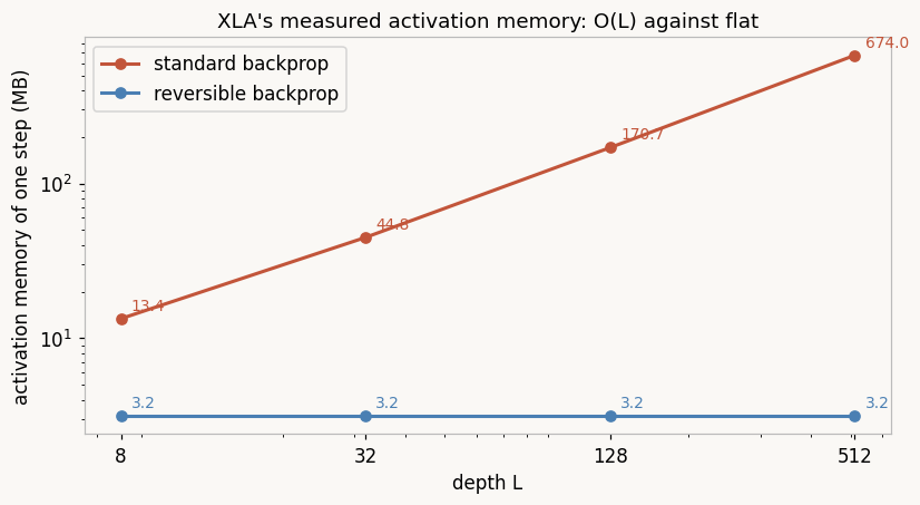
The time column is the price: the backward pass runs block once more per layer, and at depth 512 that costs 24%. Recompute for memory, the same trade RevNets built into their architecture (Gomez et al., 2017), paid here by the integrator’s own inverse (Sander et al., 2021).
The cliff, in numpy float32
The explainer’s noise budget says the rewind amplifies float error by per layer. You do not need a GPU to watch that happen; you need np.float32 and the same twenty lines:
def rewind(F, xL, vL, mu, L):
    mu = np.float32(mu)
    x, v = xL.astype(np.float32), vL.astype(np.float32)
    for _ in range(L):
        x = (x - v).astype(np.float32)
        v = ((v - field(F, x)) / mu).astype(np.float32)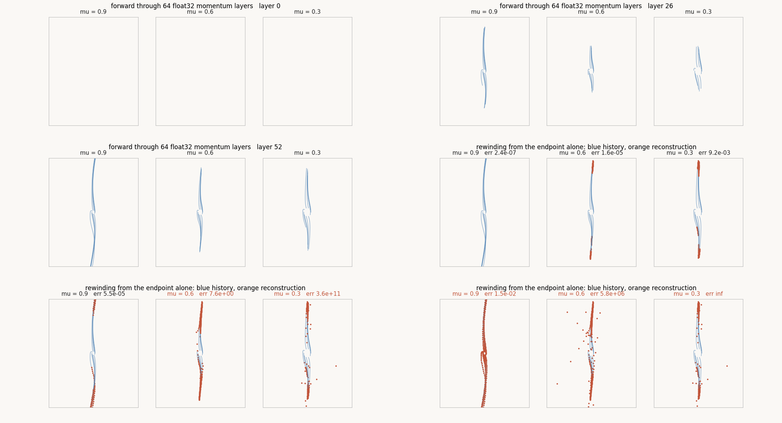
And the growth is not vaguely exponential, it is the predicted exponential. Plotting the reconstruction error as the rewind proceeds, against the budget drawn dashed:
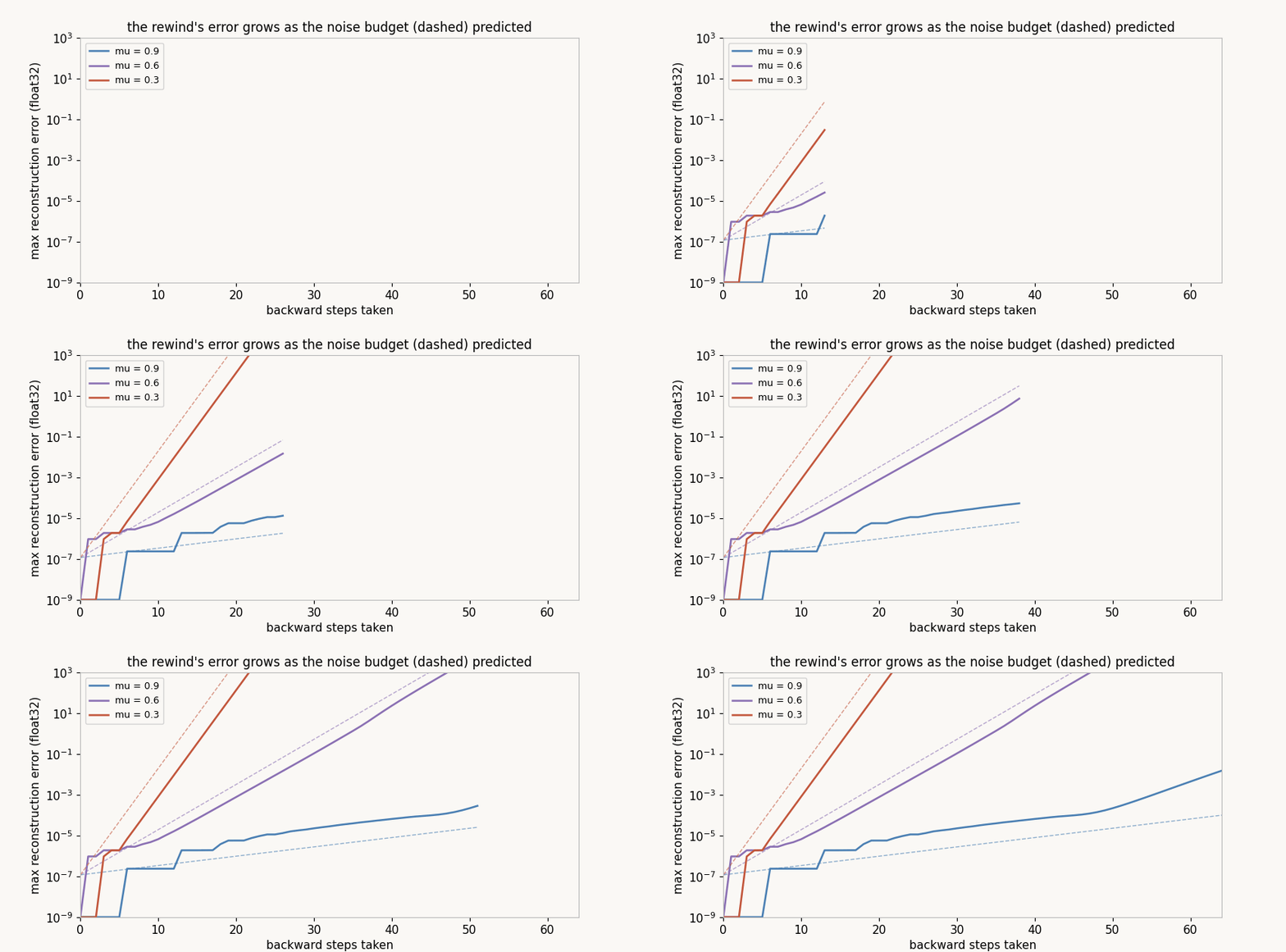
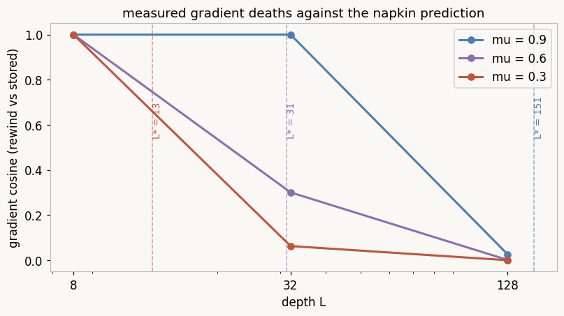
On the full network the run measures gradient agreement (cosine between the rewind gradient and the stored-activation gradient on identical weights and batch): 1.000000 everywhere the budget is small, 0.30 at , depth 32, where the budget crosses one, and nan at , depth 128, where the budget is .
Training on the rewind
Inside the budget the two gradients are the same numbers, so training should be indistinguishable up to noise, and the run checks at depth 64, : standard 81.6% test accuracy, reversible 79.7%, one seed each, reversible 17% slower on the wall. The explainer closes the loop with the architectural moral: the amplification exists because , and the frictionless leapfrog block rewinds by subtraction alone, no division, no budget, no cliff.
Every number above is from one run on Kaggle (bundle kgl_blog-revmem-v1); the float32 demonstrations are rendered from the same arithmetic the panels run live.
Cite as
Bouhsine, T. (). Reversible Backprop as a custom_vjp in JAX. Records of the !mmortal Data Scientist. https://tahabouhsine.com/blog/backprop-without-the-memory-jax-flax-nnx/
BibTeX
@misc{bouhsine2026backpropwithoutthememoryjaxflaxnnx,
  author       = {Bouhsine, Taha},
  title        = {Reversible Backprop as a custom_vjp in JAX},
  year         = {2026},
  month        = {jul},
  howpublished = {\url{https://tahabouhsine.com/blog/backprop-without-the-memory-jax-flax-nnx/}},
  note         = {Blog post, Records of the !mmortal Data Scientist}
}