A Velocity Ledger for Transformers, in JAX/Flax NNX

The explainer read a pre-norm Transformer layer $x \mathrel{+}= \mathrm{Attn}(\mathrm{norm}\,x);\ x \mathrel{+}= \mathrm{MLP}(\mathrm{norm}\,x)$ as two forward-Euler steps and asked what a velocity stream in the residual stream buys a real language model. The answer split: on quality the four variants tie, on dynamics the ledger makes the residual-stream path far shorter and straighter. This is the implementation: the plain block as Euler, the velocity ledger as one line of Flax NNX state, the ngpt-lite retraction variant, best-val early-stopped training, and the depth telemetry that measures the path. Every published number is from scripts/velocity_ledger.py; every figure is rendered from that run’s bundle by scripts/render_velocity_ledger_gifs.py.

The plain block is one Euler step#

Before any ledger, the block the whole post leans on, small enough to trust. A pre-norm Transformer layer reads a normalized copy of the residual stream, runs it through attention, adds the raw result back, and does the same with the MLP. Two sub-updates, each a state plus an increment, each forward Euler on the stream:

def plain_step(x, ln, f, mask=None):
    # x  += f(norm x):  read a normalized copy, integrate the field, write back.
    # This is one forward-Euler step on the residual stream x (Delta t = 1).
    return x + f(ln(x))

The norm is the only wrinkle the ResNet did not have: the field is integrated on a normalized copy of the stream, then the raw increment is written to the un-normalized state. That is a preconditioning of the field, not a change to the integrator. The update is still position-plus-increment. Which means, exactly as in D1, there is no velocity anywhere: each sub-update moves the stream directly and forgets the direction of the last.

The ledger is one line of state#

What does it take to give the residual stream a velocity? One persistent array, threaded through the layers, that the blocks write into instead of the stream. D1’s heavy-ball update, verbatim, now shared across both sub-updates of every layer:

def ledger_step(x, v, ln, f, mu=0.9, h=1.0, mask=None):
    # the block writes to the velocity stream; the velocity moves the state.
    # mu = 0 recovers plain_step EXACTLY. v is depth-state, not a weight: 0 params.
    v = mu * v + (1.0 - mu) * f(ln(x))
    x = x + h * v
    return x, v

At $\mu = 0$ the ledger forgets instantly and ledger_step is plain_step: one dial from Euler to heavy-ball, at identical parameter count, because $\mu$ and $h$ are fixed scalars, not learned. The velocity $v$ is depth-state (it lives only during the forward pass, zero-initialized at the embedding), so the ledger adds exactly zero parameters, verified in the bundle: plain and ledger both weigh 2,724,864 params.

Both blocks live in one Flax NNX module, and the residual stream is threaded as a plain loop over the layers. The full model in scripts/velocity_ledger.py builds the four variants from the same Block; here is the residual-stream core, the part that differs:

class Block(nnx.Module):
    def __init__(s, variant, dm, ff, heads, drop, *, rngs):
        if variant.startswith('ngpt'):
            s.alpha1 = nnx.Param(jnp.ones((dm,)))   # per-dim step scale (attn)
            s.alpha2 = nnx.Param(jnp.ones((dm,)))   # per-dim step scale (mlp)
        else:
            s.ln1 = nnx.LayerNorm(dm, rngs=rngs)
            s.ln2 = nnx.LayerNorm(dm, rngs=rngs)
        s.attn = nnx.MultiHeadAttention(num_heads=heads, in_features=dm,
                                        dropout_rate=drop, decode=False, rngs=rngs)
        s.fc1 = nnx.Linear(dm, ff, rngs=rngs)
        s.fc2 = nnx.Linear(ff, dm, rngs=rngs)
        s.drop1 = nnx.Dropout(drop, rngs=rngs)
        s.drop2 = nnx.Dropout(drop, rngs=rngs)

The stream loop, one branch per variant, is where D1’s dictionary becomes code. led toggles the velocity; ngpt toggles the sphere:

v = jnp.zeros_like(x)                       # the velocity stream, zero at embed
for b in s.blocks:
    for which in ('attn', 'mlp'):
        inp = x if ngpt else (b.ln1 if which == 'attn' else b.ln2)(x)
        f = (b.drop1(b.attn(inp, mask=mask)) if which == 'attn'
             else b.drop2(b.fc2(jax.nn.gelu(b.fc1(inp)))))
        if led:                             # the velocity ledger (heavy-ball)
            v = MU * v + (1.0 - MU) * f
            step = H_STEP * v
        else:
            step = f
        if ngpt:                            # per-dim step scale
            step = (b.alpha1 if which == 'attn' else b.alpha2).value * step
        x = x + step
        if ngpt:
            x = retract(x, math.sqrt(s.dm)) # back to the sphere of radius sqrt(D)

The sphere variant, and what it is not#

nGPT (Loshchilov et al., 2024) is the deliberate contrast: a first-order optimizer on the hypersphere, no velocity. Our ngpt-lite is a simplified version: the state is retracted to the sphere of radius $\sqrt{D}$ after the embedding and after every sub-update, the in-block LayerNorms are dropped (the state is already normalized), and the eigen learning rates become a per-layer, per-dimension learnable step scale $\alpha$. What we do not claim is full nGPT: no weight-matrix normalization, no logit scale, no QK normalization. The retraction is one line:

def retract(z, radius):
    # renormalize each token vector back onto the sphere of the given radius
    return z * (radius / (jnp.linalg.norm(z, axis=-1, keepdims=True) + 1e-8))

ngpt-ledger is the synthesis: run the heavy-ball ledger in ambient space from the block output, take the scaled step, then retract. It is the accelerated optimizer on the sphere, the natural experiment the explainer flagged.

Best-val, not the endpoint#

Two loss numbers at the end of training would mislead, because a Transformer can over-train and the endpoint measures memorization, not quality. The headline metric is the best (early-stopped) validation loss over the whole run, and it is worth writing the loop that way explicitly:

best_val = float('inf')
for it in range(1, STEPS + 1):
    x, y = get_batch('train', BATCH, seed * 1000003 + it)
    loss = step(model, opt, x, y)                 # dropout ON (model.train())
    if it % VAL_LOG == 0 or it == STEPS:
        model.eval()                              # dropout OFF for val + telemetry
        vl = np.mean([eval_loss(model, vx, vy) for vx, vy in val_batches])
        model.train()
        best_val = min(best_val, float(vl))

Run all four variants, three seeds, on the complete works of Shakespeare (character level, about 5.4M characters, so 12000 steps is roughly 14 epochs, not the 90 that memorized an earlier tinyshakespeare run). The four converge on top of each other:

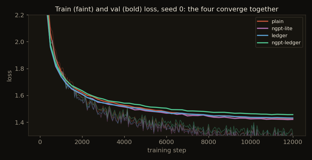
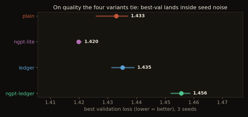
Across three seeds the best-val numbers are a tie: plain 1.433, ledger 1.435, ngpt-lite 1.420, ngpt-ledger 1.456, a spread of 0.036 against a per-seed noise of about 0.005. The velocity ledger did not move quality.

The telemetry that finds the signal#

If the four tie on quality, the interesting question is what they do differently to get there, and D1 already told us where to look: the geometry of the residual-stream path. The telemetry runs the field on a fixed probe batch (dropout off) and, at each of four checkpoints, records the per-sub-update displacement and the turning angle:

def depth_stats(model, probe):
    _, rec = model._stream(probe, collect=True)         # collect x at every node
    xs = np.stack([np.asarray(a) for a in rec['x']])    # [2L+1, B, T, D]
    seg = np.diff(xs, axis=0)                            # per-sub-update step
    seglen = np.linalg.norm(seg, axis=-1)               # path length per step
    d1, d2 = seg[:-1], seg[1:]
    cos = (d1 * d2).sum(-1) / (np.linalg.norm(d1, -1) * np.linalg.norm(d2, -1) + 1e-12)
    turn = np.degrees(np.arccos(np.clip(cos, -1, 1)))   # turning angle per step
    return {'seglen': seglen.mean((1, 2)), 'turn': turn.mean((1, 2)), ...}

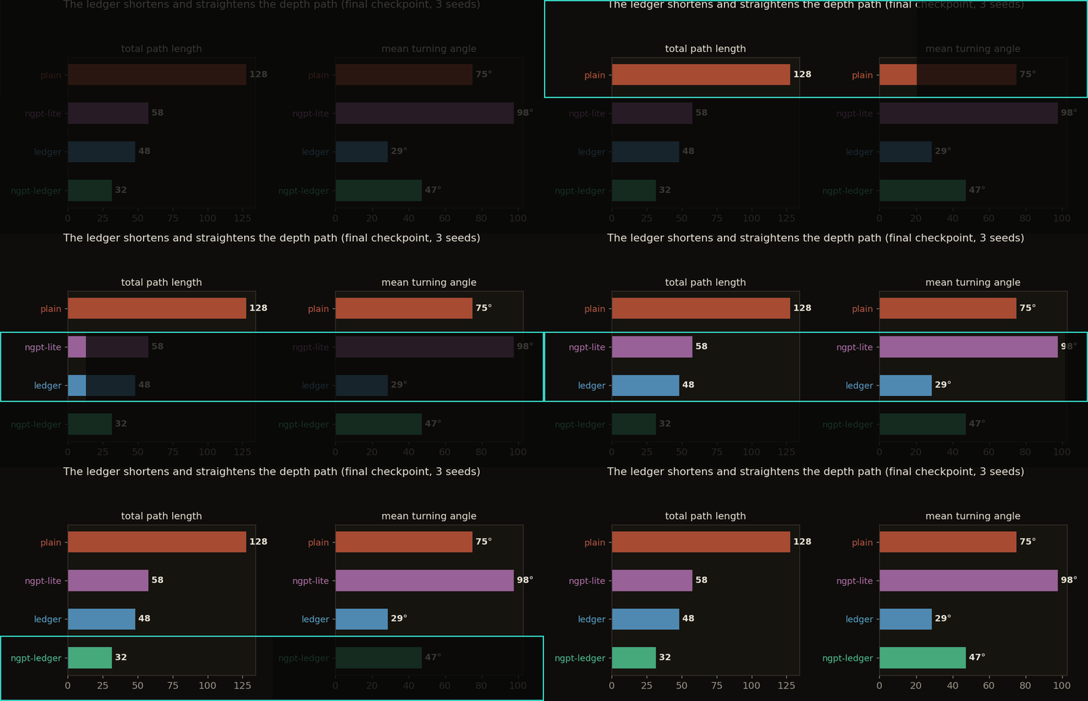
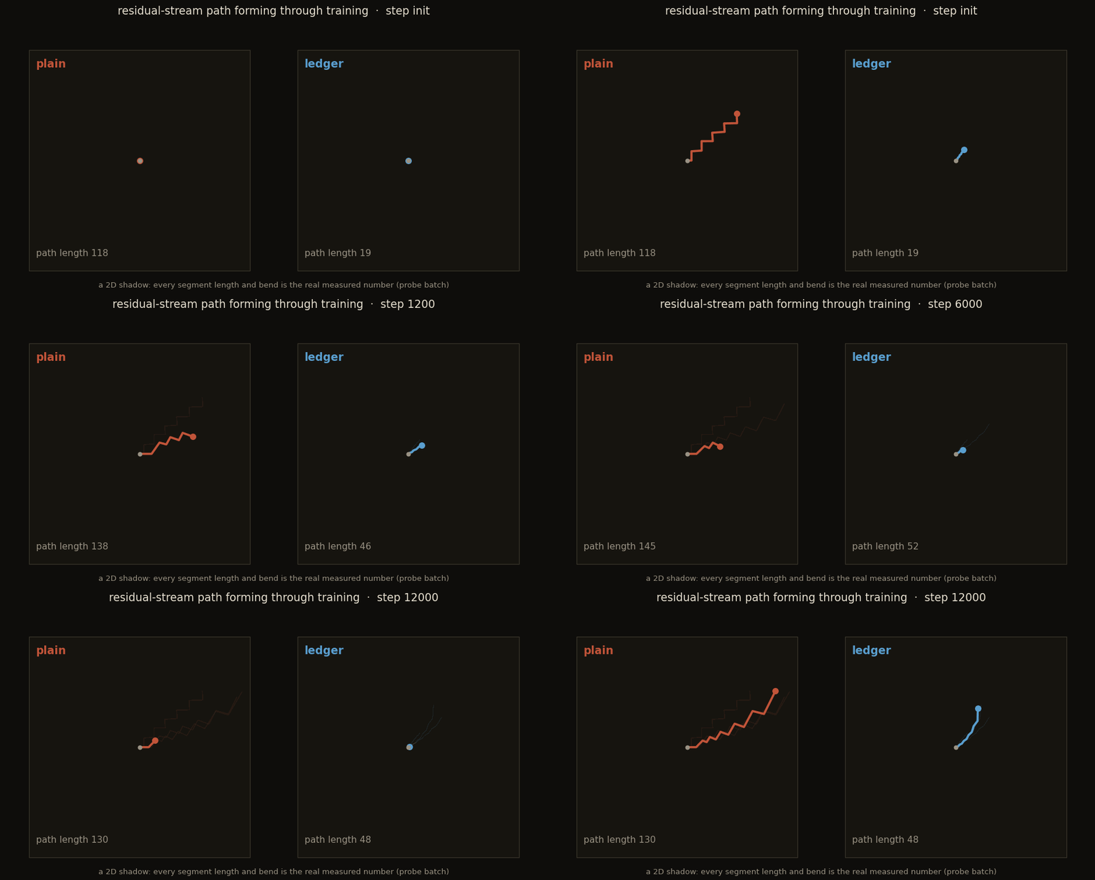
Summed over the twelve sub-updates, the total path lengths (3-seed mean, final checkpoint) separate cleanly: plain 128, ngpt-lite 58, ledger 48, ngpt-ledger 32. The turning angles do too: plain 75 degrees a step, ledger 29, ngpt-lite 98, ngpt-ledger 47. The velocity ledger cuts the path to roughly a third and the sharpness to under half, at a tied best-val.

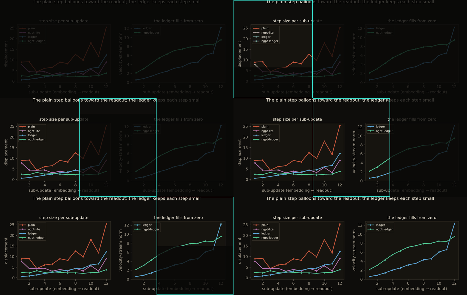
The mechanism is the $(1-\mu)$ damping: a plain layer writes the full block output into the stream, while the ledger writes a running average of it, so no single block output can move the state far. Watch the step sizes and the velocity that funds them:

The path straightening, as it happens#

The one thing here that is a real process is how the path changes over training. All four start short at initialization (an untrained field is small); training is what pushes the plain net’s path out into a long wander while the ledger holds its short. The telemetry was dumped at four checkpoints, so we can watch the two paths form, side by side, and watch the gap open:

What carried over#

D1’s prediction transferred to a Transformer and held, at the level where it actually applies. The pre-norm block is forward Euler on the residual stream; the velocity ledger is one line of NNX state and zero parameters; and at $\mu = 0$ it collapses exactly to the plain block. On this small char-level GPT it does not move quality, the four variants tie on best-val to within seed noise, and it is not an upgrade. What it moves is the dynamics: the residual stream reaches an equally-good answer along a path a third as long (48 against 128 units) and less than half as sharp (29 against 75 degrees a step), whether the geometry is flat or spherical. A skip connection is half of Newton in a Transformer too, and the other half is a calmer, straighter path to the same destination.

The four residual-stream updates and their telemetry are from scripts/velocity_ledger.py (JAX + Flax NNX, run once on Kaggle); the momentum residual network the ledger borrows is from Sander et al. (2021); the hypersphere variant is a simplified nGPT; the depth-as-dynamics reading of Transformers is Lu et al. (2019). The conceptual companion is Transformers With a Velocity Ledger.

@misc{bouhsine2026transformerswithavelocityledgerjaxflaxnnx,
  author       = {Bouhsine, Taha},
  title        = {A Velocity Ledger for Transformers, in JAX/Flax NNX},
  year         = {2026},
  month        = {jul},
  howpublished = {\url{https://tahabouhsine.com/blog/transformers-with-a-velocity-ledger-jax-flax-nnx/}},
  note         = {Blog post, Records of the !mmortal Data Scientist}
}