Skip Connections With Inertia, in JAX/Flax NNX
#ml#resnet#momentum-resnet#neural-ode#jax#flax#nnx#implementation#dynamical-systems#symplectic-integrators#deep-learning
Part 1 of 5Networks as Integrators
Hand the trained network only its own output and ask for its input back. In double precision it comes home to the thirteenth decimal. In single precision, with the friction turned from 0.9 down to 0.3, the same loop returns garbage. Nothing in the formula changes between those two runs, and working out what does is the sharpest thing in this companion. The explainer reads a residual block as one forward-Euler step and asks what a velocity state buys; below are the two integrators in eight lines apiece, the momentum residual network as a Flax NNX module with one extra line of state, the rings task a first-order flow cannot separate exactly, and the rewind.
Prefer a notebook? Run the whole thing on Kaggle: the same code, block by block, with the math written out and every figure reproduced from a real run.
Two integrators, eight lines apart
Before any network, the physics fact the whole post leans on, in code small enough to trust. A second-order system carries two states, position and velocity. Forward Euler updates both from the stale state; leapfrog interleaves them, half a velocity kick, a position drift with the fresh velocity, half a kick to finish. Same force, same step size:
def accel(r):                                  # Kepler, GM = 1
    return -r / np.linalg.norm(r) ** 3

def euler(r, v, dt):
    a = accel(r)
    return r + dt * v, v + dt * a              # both updates from the stale state

def leapfrog(r, v, dt):
    v = v + 0.5 * dt * accel(r)                # half kick
    r = r + dt * v                             # drift with the FRESH velocity
    return r, v + 0.5 * dt * accel(r)          # half kick
Before anyone bills leapfrog double, one accounting note: as written, leapfrog calls accel twice per step where euler calls it once, because this version favors visible symmetry over bookkeeping. In the standard kick-drift-kick formulation the force that closes one step is exactly the force that opens the next, so a production integrator caches it and the steady-state cost is one force evaluation per step, the same as Euler.
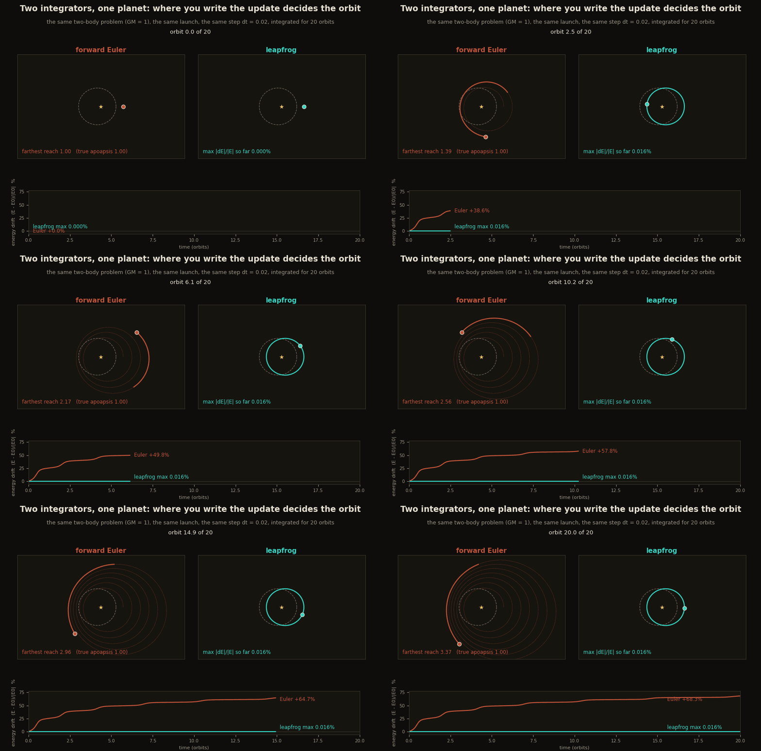
Launch the same planet with both, , twenty orbits, and print the damage:
Euler:    energy drift +68.3% over 20 orbits, farthest reach 3.37
leapfrog: max energy deviation 0.016%
Euler injects a sliver of energy on the outside of every curve, and twenty orbits later the ellipse with apoapsis reaches out to and is still swelling. Leapfrog’s error breathes but never accumulates. Nothing about the force changed; only where the update is written down.
One module, one dial
What does it take to give a residual network the second ledger? One line of state. The momentum residual network of Sander et al. (2021) writes the block’s output into a velocity, damped by a friction , and lets the velocity move the state:
At the ledger forgets instantly and this is the plain residual network , forward Euler on the field . One module covers both architectures, at identical parameter count, because is a fixed scalar, not a weight:
class MomentumResNet(nnx.Module):
    """v' = mu v + (1 - mu) F_l(x);  x' = x + h v'.  At mu = 0 this IS the
    plain residual network x' = x + h F_l(x): one dial from Euler to Newton."""

    def __init__(self, L=32, width=2, hidden=16, mu=0.9, T=8.0, *, rngs):
        gain1 = nnx.initializers.normal(1.0 / math.sqrt(width))
        gain2 = nnx.initializers.normal(1.0 / math.sqrt(hidden))
        self.blocks = [(nnx.Linear(width, hidden, kernel_init=gain1, rngs=rngs),
                        nnx.Linear(hidden, width, kernel_init=gain2, rngs=rngs))
                       for _ in range(L)]
        self.readout = nnx.Linear(width, 2, kernel_init=gain1, rngs=rngs)
        self.mu, self.h = mu, T / L

    def __call__(self, x, return_state=False):
        v = jnp.zeros_like(x)
        for lin1, lin2 in self.blocks:
            f = lin2(jnp.tanh(lin1(x)))            # the vector field F_l(x)
            v = self.mu * v + (1 - self.mu) * f    # the block writes to the LEDGER
            x = x + self.h * v                     # the ledger moves the state
        return (self.readout(x), x, v) if return_state else self.readout(x)
Two decisions in the constructor matter for everything downstream. The residual stream is width 2, so the hidden state is a literal point in a plane and every trajectory in this post is the state itself, not a projection. And the total integration time is fixed at , so depth refines the same flow: means steps of . The blocks are per-layer (untied), a tiny tanh MLP each, the explainer’s setup unchanged.
Training on the task a flow cannot get exactly right
The interesting dataset is the one the physics singled out: a disk of one class walled in by an annulus of the other. A first-order planar flow is a homeomorphism, its trajectories cannot cross, so it can never pull the inside class out exactly; a network with a velocity state doubles the state to and crosses freely in the position shadow. Rings are ten lines:
def make_rings(n, rng, noise=0.04):
    """Class 0 is a disk; class 1 is an annulus that walls it in at every angle."""
    n2 = n // 2
    th, r_in = rng.uniform(0, 2 * np.pi, n2), 0.6 * np.sqrt(rng.uniform(0, 1, n2))
    th2, r_out = rng.uniform(0, 2 * np.pi, n2), rng.uniform(1.3, 1.8, n2)
    X = np.concatenate([np.stack([r_in * np.cos(th), r_in * np.sin(th)], 1),
                        np.stack([r_out * np.cos(th2), r_out * np.sin(th2)], 1)])
    X += rng.normal(0, noise, X.shape)
    y = np.repeat(np.arange(2), n2).astype(np.int32)
    return X.astype(np.float32), y
The training loop is standard NNX, full-batch Adam, 4000 steps, a linear readout on the final 2-D state:
def train(mu, seed=0, steps=4000):
    rng = np.random.default_rng(1000 + seed)
    Xtr, ytr = map(jnp.asarray, make_rings(1024, rng))
    Xte, yte = map(jnp.asarray, make_rings(2048, rng))
    model = MomentumResNet(mu=mu, rngs=nnx.Rngs(seed))
    opt = nnx.Optimizer(model, optax.adam(3e-3), wrt=nnx.Param)

    @nnx.jit
    def step(model, opt):
        def loss_fn(m):
            return optax.softmax_cross_entropy_with_integer_labels(m(Xtr), ytr).mean()
        loss, grads = nnx.value_and_grad(loss_fn)(model)
        opt.update(model, grads)
        return loss

    for _ in range(steps):
        loss = step(model, opt)
    acc = (model(Xte).argmax(1) == yte).mean()
    return model, Xte, float(acc)
rings, L=32, mu=0.0: test accuracy 99.80%
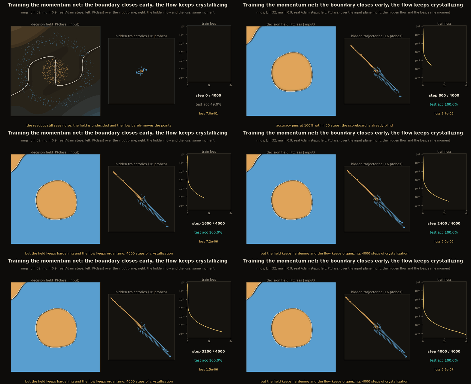
rings, L=32, mu=0.9: test accuracy 100.00%Watch that training happen rather than take the two numbers. The run below is the momentum net’s, dumped every 50 steps: the decision field over the input plane, the hidden trajectories, and the loss, all at the same moment. The striking part is the timing. Accuracy pins at 100% within the first 50 steps, and then the network spends 3,950 more steps reorganizing anyway: the boundary hardens, the probability mass polarizes, the hidden flow straightens. The scoreboard stopped watching long before the dynamics stopped moving.
The ceiling, measured
Two training runs is not a result. The 99.80% against 100.00% above is one seed at one depth, and before reading anything into a fifth of a point, two questions have to survive the full sweep: does the gap hold across three seeds and three depths, and does a plain net that is deep enough to be a true flow ever touch the 100% line at all? The sweep’s first answer is a null. There is no cliff anywhere in it: on two moons both rules sit between 99.85% and 100% everywhere, and even on rings the plain net at depth 128 posts 99.85% on average.
What the theorem forbids is exactness, and exactness is the one line in the figure that matters: which dots ever touch the dashed 100% line.
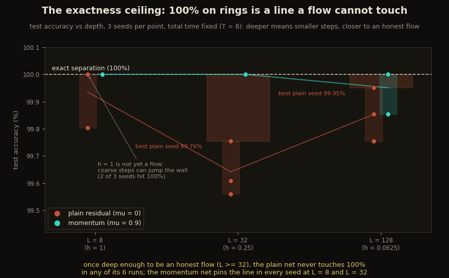
The seed accounting behind the dots: at depth 8 the plain net is not yet a flow (steps of can jump the wall) and it hits 100.0% in two seeds of three; at depths 32 and 128, where it refines into a true flow, it never touches 100% again in any of its six runs, its best seeds stalling at 99.76% and 99.95%, while the momentum net pins 100.0% in every seed at depths 8 and 32. On spirals the same ledger shows up as reliability rather than a ceiling: the plain net’s three depth-128 seeds spread from 92.9% to 98.3%, the momentum net’s sit within six tenths of a point of each other.
The whole sweep fits in one table, so the plot above can be audited at a glance: three seeds per cell, mean test accuracy with the min-to-max seed range in parentheses.
| task | depth | plain net, (%) | momentum net, (%) |
|---|---|---|---|
| moons | 8 | 99.97 (99.95 to 100.0) | 99.98 (99.95 to 100.0) |
| moons | 32 | 99.85 (99.80 to 99.95) | 99.98 (99.95 to 100.0) |
| moons | 128 | 99.89 (99.80 to 100.0) | 99.97 (99.90 to 100.0) |
| spirals | 8 | 96.18 (94.87 to 97.61) | 97.66 (96.88 to 98.44) |
| spirals | 32 | 97.82 (97.36 to 98.44) | 97.54 (97.22 to 97.75) |
| spirals | 128 | 96.16 (92.87 to 98.29) | 98.08 (97.71 to 98.34) |
| rings | 8 | 99.93 (99.80 to 100.0) | 100.00 (100.0 in all seeds) |
| rings | 32 | 99.64 (99.56 to 99.76) | 100.00 (100.0 in all seeds) |
| rings | 128 | 99.85 (99.76 to 99.95) | 99.95 (99.85 to 100.0) |
The 1890s uniqueness theorem did not predict a collapse; it predicted a ceiling, and the ceiling is where the runs put it. A homeomorphism cornered by topology squeezes the surrounding class into a thin filament, hides its mistakes inside it, and pays a stray handful of test points as rent, forever.
Watching the state instead of the scoreboard
Two networks separated by a tenth of a point on the scoreboard are doing violently different things underneath, and with a width-2 stream we can just look. The exported hidden trajectories of the two trained depth-32 rings nets, the same states the explainer’s panels integrate, play out below, block by block.
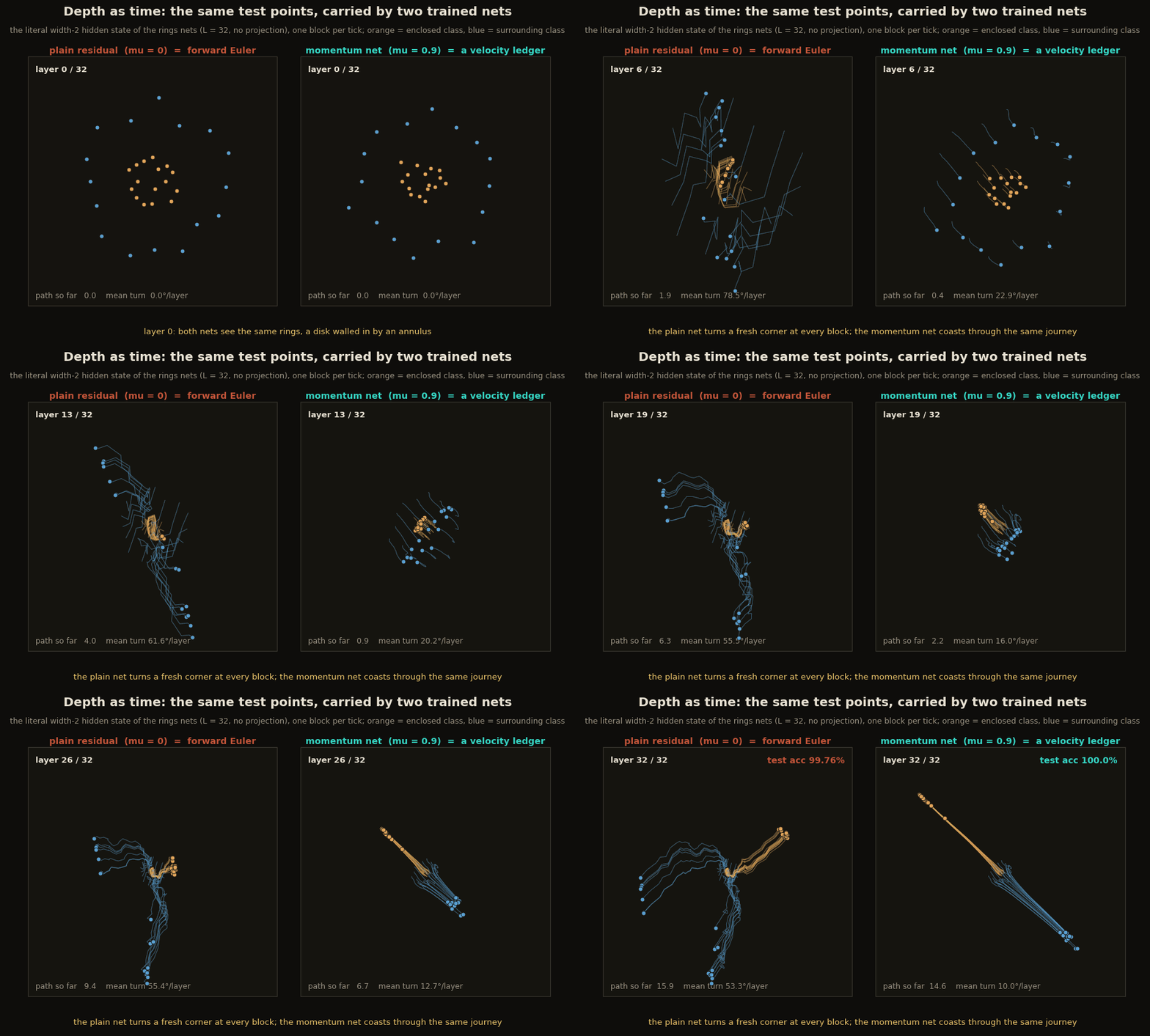
That is Prediction 1 of the explainer on real weights: Euler trajectories turn as sharply as the local field because every step forgets the last one; momentum trajectories coast through turns, overshoot slightly, and curve back, the way things with mass move.
The ledger, made visible
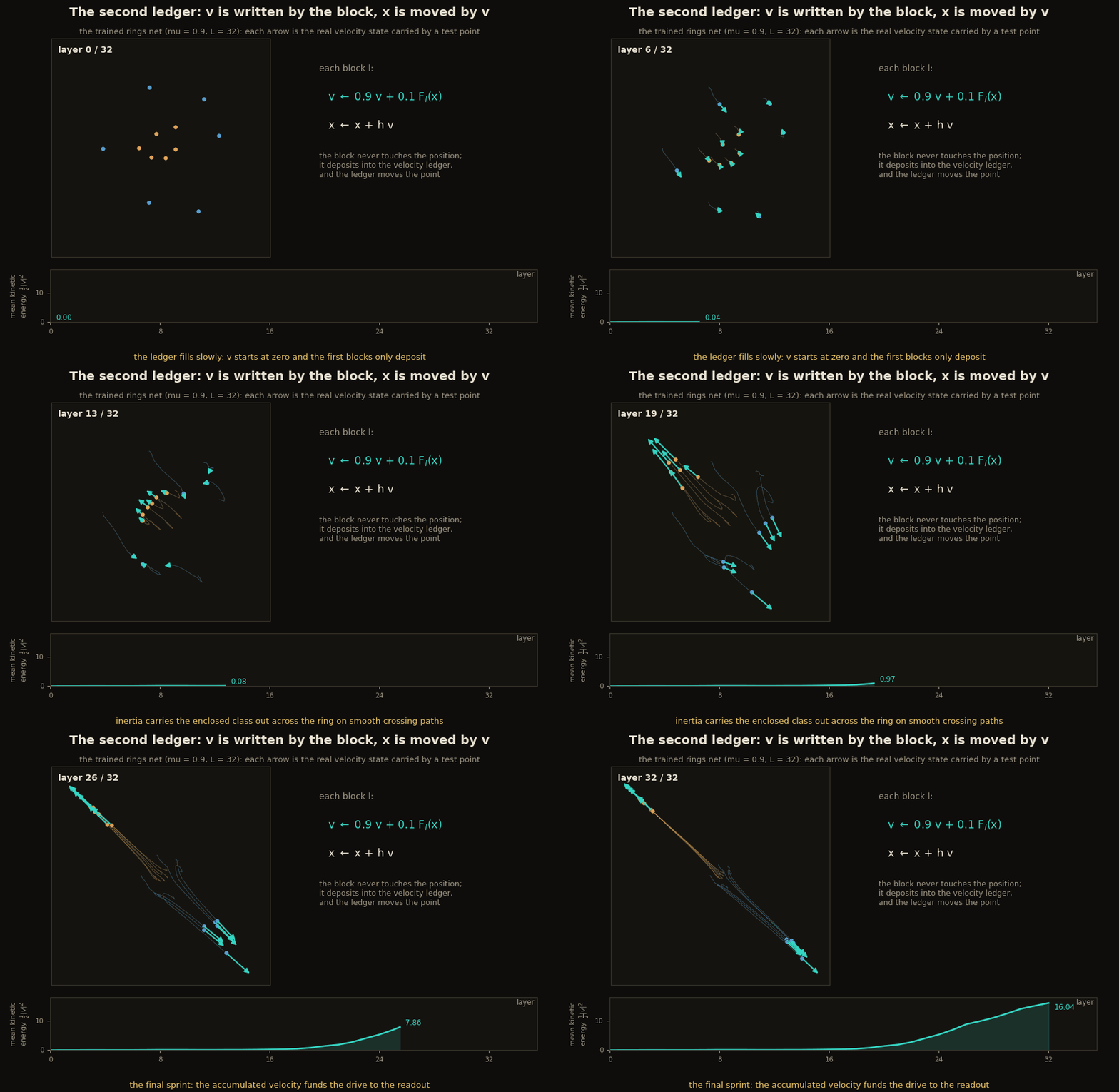
The velocity state itself is worth seeing, because it is the whole mechanism and it never appears on any scoreboard. Run the trained net forward, keep the ledger’s value at every block, and draw as an arrow on every point:
Running the whole network backward
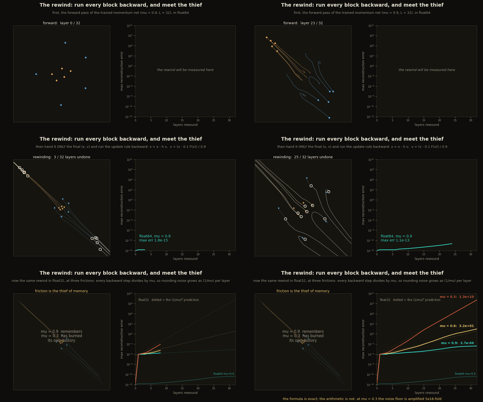
Now the strangest property, and the reason Sander et al. built these networks in the first place. The update rule is algebraically invertible: given the final , each block can solve for its own past, no stored activations anywhere:
def rewind(model, xL, vL):
    """From the final (x, v) alone, solve every block for its own past."""
    x, v = xL, vL
    for lin1, lin2 in reversed(model.blocks):
        x = x - model.h * v                        # undo the drift
        f = lin2(jnp.tanh(lin1(x)))
        v = (v - (1 - model.mu) * f) / model.mu    # undo the deposit: divide by mu
    return x, v
Try to write this for the plain block and you can’t: overwrote its own input, and recovering it means solving a nonlinear equation with no uniqueness guarantee. The velocity is the receipt that makes the computation reversible.
Run it on the trained net, in double precision, and the receipt is honored to the last digit:
rewind mu=0.9 float64: max |x0_rec - x0| = 5.8e-13Sixty-four test points pushed through thirty-two blocks and pulled back out, reconstructed to . But run the same loop in single precision, and then turn the friction up, and something far more instructive happens:
rewind mu=0.9 float32: max |x0_rec - x0| = 3.3e-04
rewind mu=0.6 float32: max |x0_rec - x0| = 1.7e+02
rewind mu=0.3 float32: max |x0_rec - x0| = 9.7e+09
Nothing is wrong with the formula. Look at the last line of rewind: every backward step divides by , so whatever rounding noise the forward pass left behind is amplified by per layer. At that is a factor of across 32 layers, gentle enough that single precision still comes home to . At it is a factor of , and the past is simply gone. The explainer’s canonical run measures the same law on its single-precision forward pass: at , at , at . The friction dial is a memory dial: a lightly damped system can be rewound, a heavily damped one has burned its own history, and floating point is just the messenger. None of this is news to the architects: Sander et al. (2021) discuss precisely this finite-precision leak, and their exactly-invertible implementation stores the low-order bits each forward update would discard so the backward pass can hand them back. The three error lines above are the reason that bookkeeping exists.
This is not a party trick. A network you can run backward is a network you can train without caching activations: recompute each block’s input from its output during the backward pass, and the memory cost of depth almost vanishes. That is the engineering payoff Sander et al. (2021) built Momentum ResNets around, and it falls out of the same physics that keeps the leapfrog planet on its ellipse: time-reversible integrators conserve the information the rewind needs, and is the dial that decides how much of it survives arithmetic.
What carried over
Every claim the explainer made on physics grounds survived contact with real trained weights, in about a hundred lines of NNX. The plain residual block is forward Euler, and it kinks (52.9 degrees per layer) where the momentum block coasts (9.6). The missing second state is one line of module code, costs zero parameters, and buys crossing trajectories where topology forbids a flow to go: the plain net never touches 100% on rings once it is deep enough to be a true flow, and the momentum net pins it. At every scale the scoreboard was blind to the ledger: across architectures, across , and inside a single run, where accuracy pinned at step 50 and the dynamics kept crystallizing for 3,950 more. And the ledger’s damping is exactly friction, right down to which networks can remember their own past. Architecture choices are integrator choices; the numerical-analysis shelf is full of integrators nobody has read as networks yet.
The momentum residual network is from Sander et al. (2021); depth-as-time from Chen et al. (2018); the non-crossing obstruction as a network ceiling from Dupont et al. (2019); the geometry of why leapfrog holds its orbit from Hairer, Lubich and Wanner (2006). The conceptual companion is Your Skip Connection Is Half of Newton.
Cite as
Bouhsine, T. (). Skip Connections With Inertia, in JAX/Flax NNX. Records of the !mmortal Data Scientist. https://tahabouhsine.com/blog/momentum-resnet-jax-flax-nnx/
BibTeX
@misc{bouhsine2026momentumresnetjaxflaxnnx,
  author       = {Bouhsine, Taha},
  title        = {Skip Connections With Inertia, in JAX/Flax NNX},
  year         = {2026},
  month        = {jul},
  howpublished = {\url{https://tahabouhsine.com/blog/momentum-resnet-jax-flax-nnx/}},
  note         = {Blog post, Records of the !mmortal Data Scientist}
}References
- (2021). Momentum Residual Neural Networks. ICML 2021.arXiv:2102.07870
- (2018). Neural Ordinary Differential Equations. NeurIPS 2018.arXiv:1806.07366
- (2019). Augmented Neural ODEs. NeurIPS 2019.arXiv:1904.01681
- (2006). Geometric Numerical Integration: Structure-Preserving Algorithms for Ordinary Differential Equations. Springer, 2nd ed..