Editing a Deep Equilibrium Network, in JAX/Flax NNX

The most important diagnostic in this file is a short power iteration called local_slope. It reports the operator’s largest local slope at each observed fixed point, and the natural class edit sends the maximum from 0.904 to 1.438. That loss of local margin is a reason to temper the edit and probe the solver again, not a global theorem about every state. The explainer works out why editability splits in two once a stack melts into a single iterated operator; here are both edits, the gain audit, and the drift of 520 old fixed points.

Prefer a notebook? Run the whole thing on Kaggle: the same code, block by block, with the math written out and every figure reproduced from a real run.

The operator, as one shared module#

If an edit is going to reach every depth at once, there has to be only one thing to edit. The whole network is a single Yat operator on a 32-dimensional state, iterated from zero until it stops. The prototypes are the rows of W, the mixing matrix A sends their scores back into the state, and there is no per-layer anything: the same module is applied over and over, so its rows are present at every turn by construction.

import jax, jax.numpy as jnp
from jax import lax
from flax import nnx

class YatDEQ(nnx.Module):
    """One shared Yat operator F(z;x) = tanh(A·φ_W(z) + U·x + z0), iterated to z* = F(z*;x)."""
    def __init__(self, W, A, Uin, z0, C, cb, *, b=0.5, eps=1.0, beta=0.7, iters=200):
        self.W  = nnx.Param(jnp.asarray(W))       # [M, 32]  shared prototype bank
        self.A  = nnx.Param(jnp.asarray(A))       # [32, M]  mixing: scores back into the state
        self.Uin = nnx.Param(jnp.asarray(Uin))    # [32, 2]  input injection
        self.z0 = nnx.Param(jnp.asarray(z0))      # [32]     bias
        self.C  = nnx.Param(jnp.asarray(C))       # [ncls, 32] linear readout
        self.cb = nnx.Param(jnp.asarray(cb))
        self.b, self.eps, self.beta, self.iters = b, eps, beta, iters

    def kernel(self, z, W):                        # the Yat feature map φ_W(z), one column per prototype
        dot = z @ W.T
        d2 = (z ** 2).sum(-1, keepdims=True) + (W ** 2).sum(-1) - 2 * dot
        return (dot + self.b) ** 2 / (d2 + self.eps)

    def F(self, x, z):                             # one application of the shared operator
        return jnp.tanh(self.kernel(z, self.W.value) @ self.A.value.T + x @ self.Uin.value.T + self.z0.value)

    def zstar(self, x):                            # solve the fixed point by damped iteration
        z = jnp.zeros((x.shape[0], self.W.value.shape[1]))
        def step(z, _): return (1 - self.beta) * z + self.beta * self.F(x, z), None
        z, _ = lax.scan(step, z, None, length=self.iters)
        return z

    def __call__(self, x):                         # read the settled state linearly
        return self.zstar(x) @ self.C.value.T + self.cb.value

There is no nnx.Linear stack and no depth index anywhere in it. F is the entire network; zstar runs it until the state stops moving; __call__ reads that resting place. This is the operator the explainer trained on two interleaving moons and one Gaussian blob, three classes, 1,733 parameters shared across depth, landing at 97.9 / 98.1 / 100% per-class recall. At the observed test equilibria, the local Jacobian norm has mean 0.629 and max 0.904. Multiple-start tests then probe whether the solver returns to the same basin.

The anatomy offers exactly two places to put new rows, and the whole post is the difference between them. There are the rows that read the settled state (the readout C) and the rows that steer it (the bank W inside F). Editing the first leaves the equation alone. Editing the second edits the equation, at every depth at once.

Teach by readout: a concatenate that touches nothing#

The timid door comes with a proof, so take it first. To teach a fourth class the operator has never seen, drop eight of its examples into the frozen network, let the operator iterate them to their equilibria, and keep those settled states as anchor rows. Score the new class through the very same Yat kernel the operator uses, and paste the result on as a readout. No gradient steps.

def teach_readout(model, teach_x, alpha):
    """T1: append the taught class as a readout scored by the same Yat kernel. F untouched."""
    anchors = model.zstar(teach_x)                 # 8 equilibria = where the flow already parks the class
    def scores(x):
        z = model.zstar(x)
        old = z @ model.C.value.T + model.cb.value
        new = alpha * model.kernel(z, anchors).max(-1)   # nearest-anchor Yat score, one calibration knob
        return jnp.concatenate([old, new[:, None]], -1)
    return scores, anchors

scores, anchors = teach_readout(model, teach_x, alpha)
s = scores(Xte)
new_recall = float((s[yte == 3].argmax(-1) == 3).mean())
print("new class recall:", round(new_recall * 100, 1))            # 85.8

# the old scores are the identical computation, because F never moved
before = model(Xte_old)
after = scores(Xte_old)[:, :3]
print("max |Δ old logit|:", float(jnp.abs(after - before).max()))  # exactly 0.0

The new class is recognized at 85.8%, and the old classes are not approximately preserved, they are the identical computation: the operator was never touched, so every old fixed point and score is bit-for-bit what it was, max |Δ old logit| = 0.0, and zero old test points get captured by the new class. This is the list network’s append-a-row, alive inside the recursion.

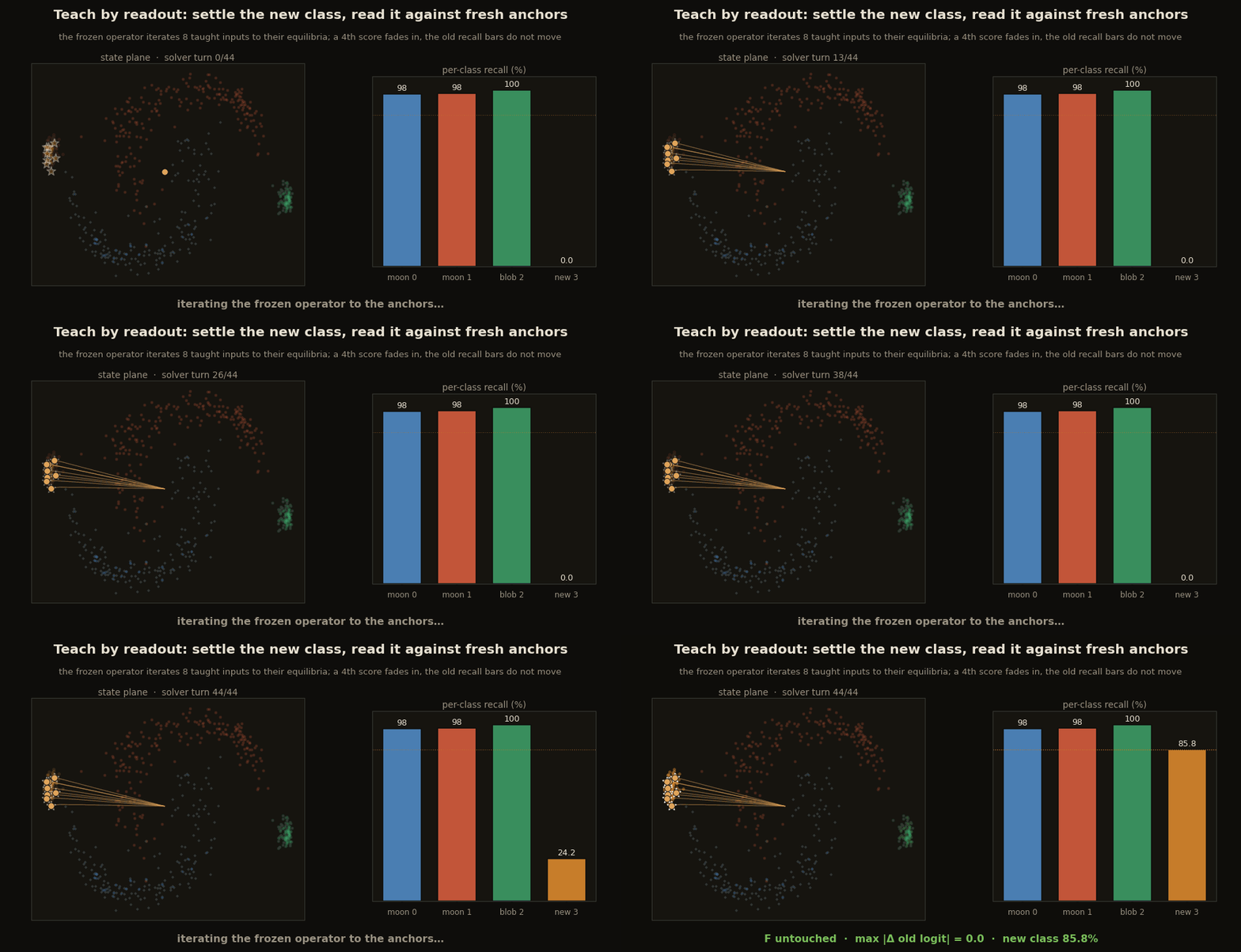
The catch is the flipside of the same fact: a readout hung beside the landscape cannot break it, but it cannot help it either. The new class’s inputs settle wherever the old flow happens to drop them, and the flow was never carved for them. The margin over the old scores is a thin 0.55, and the inputs settle a mean 0.159 from their nearest anchor, a loose cloud. To do better the mass has to go into the landscape.

Teach by dynamics: one paste, present at every depth#

The strong door drops the same anchors into the shared bank, with mixing columns that deepen a well at the new class inside the operator itself. Because there is one operator, the well is present at every turn for free. It is a jnp.concatenate on W and A.

def dyn_edit(model, anchors, gamma):
    """T2: append anchors to the shared bank with A columns γ·ĉ_k, deepening a well at every depth."""
    cols = gamma * (anchors / jnp.linalg.norm(anchors, axis=-1, keepdims=True))
    edited = nnx.clone(model)
    edited.W = nnx.Param(jnp.concatenate([model.W.value, anchors], 0))
    edited.A = nnx.Param(jnp.concatenate([model.A.value, cols.T], 1))
    return edited

That is the entire operation, and it works spectacularly better than the readout alone: with the gain tempered (the next section), the new-class recall goes 85.8% to 100%, the margin fattens from 0.55 to 3.83, and the settle distance to the nearest anchor tightens from 0.159 to 0.097. The flow now carries the new class’s inputs home instead of merely labeling where they stall. What it puts at risk is the property the whole model stands on.

The local stability audit, as a few lines of power iteration#

What could go wrong with deepening a well? In a recursion the pasted rows feed their own output back into their own input. Make the well too deep and the local slope of F can cross one around the equilibria the solver visits. The diagnostic below measures that slope: the top singular value of the operator’s Jacobian at each observed fixed point, computed by power iteration on $J^\top J$ without forming the matrix. A global contraction certificate would additionally require a uniform bound over the state domain.

def local_slope(model, x, iters=24, key=jax.random.PRNGKey(7)):
    """Per-input ‖J_F‖₂ at z* by power iteration on JᵀJ, using jvp/vjp (no matrix formed)."""
    z = model.zstar(x)
    fz = lambda zz: model.F(x, zz)
    v = jax.random.normal(key, z.shape)
    v = v / (jnp.linalg.norm(v, axis=-1, keepdims=True) + 1e-9)
    def pit(v, _):
        Jv = jax.jvp(fz, (z,), (v,))[1]                    # J v
        _, vjp = jax.vjp(fz, z); JtJv = vjp(Jv)[0]         # Jᵀ (J v)
        return JtJv / (jnp.linalg.norm(JtJv, axis=-1, keepdims=True) + 1e-9), None
    v, _ = lax.scan(pit, v, None, length=iters)
    Jv = jax.jvp(fz, (z,), (v,))[1]
    return jnp.linalg.norm(Jv, axis=-1)                    # ‖J_F‖₂ per input

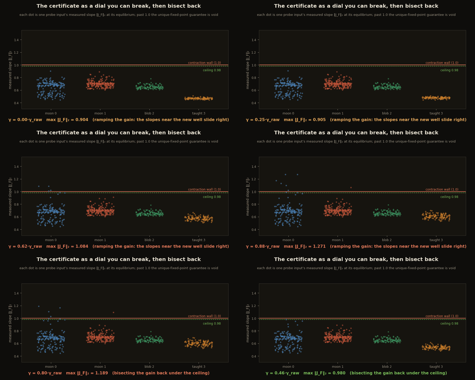
The natural paste breaks the measured local margin. Choosing $\gamma$ so each anchor gets a healthy pre-activation bump sends the maximum slope to 1.438 over the test probes. The raw edit is therefore too aggressive for the operating region the solver has demonstrated.

raw = dyn_edit(model, anchors, gamma_raw)
print("raw edit  max ‖J_F‖₂:", round(float(local_slope(raw, Xte).max()), 3))   # 1.438

The repair is one number. The edit has a single gain knob, so bisect it: find the largest fraction of the raw $\gamma$ whose measured slope stays under a ceiling of 0.98, a hair of safety below one.

def rescue_gamma(model, anchors, gamma_raw, ceiling=0.98, steps=14):
    lo, hi = 0.0, 1.0
    for _ in range(steps):
        mid = (lo + hi) / 2
        smax = local_slope(dyn_edit(model, anchors, gamma_raw * mid), Xte).max()
        lo, hi = (mid, hi) if smax < ceiling else (lo, mid)
    return gamma_raw * lo

gamma = rescue_gamma(model, anchors, gamma_raw)
edited = dyn_edit(model, anchors, gamma)                   # γ ← 0.462·γ_raw
print("tempered  max ‖J_F‖₂:", round(float(local_slope(edited, Xte).max()), 3))  # 0.980 on probes

The bisection lands on 0.462 of the raw gain. The local audit reads mean 0.646, max 0.980 over the probes, restoring the chosen empirical operating margin.

Audit the drift: 520 fixed points, re-solved and subtracted#

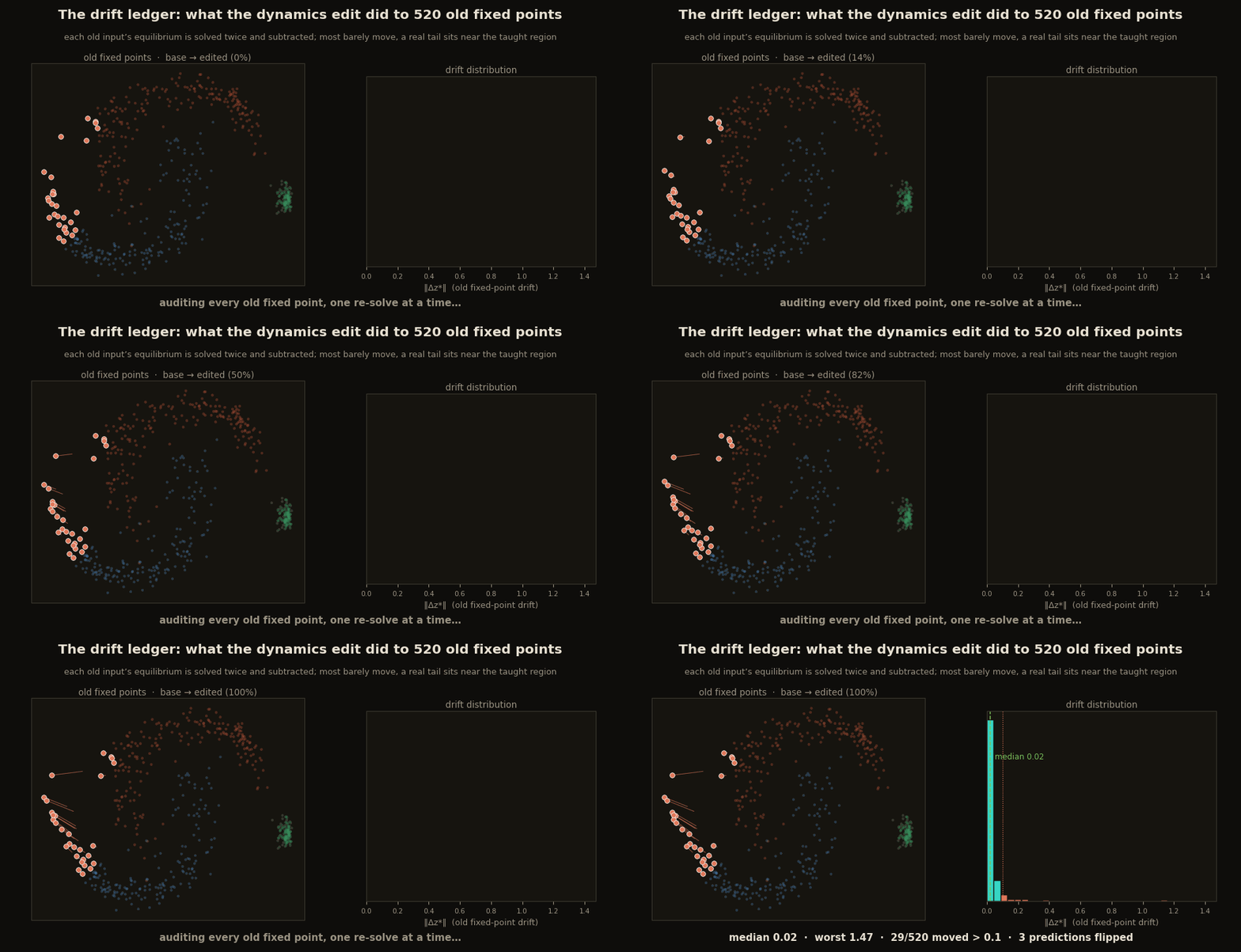
The readout edit’s invariance was a proof. The dynamics edit’s cannot be, the map moved, so what remains is a measurement, and it is the payoff of using a recursion at all: solve every old fixed point under the base operator and under the edited one, and subtract.

zb = model.zstar(Xte_old)                                  # 520 base equilibria
ze = edited.zstar(Xte_old)                                 # the same inputs, edited operator
dz = jnp.linalg.norm(ze - zb, axis=1)
print("drift  median:", round(float(jnp.median(dz)), 3),   # 0.020
      " p90:", round(float(jnp.percentile(dz, 90)), 3),    # 0.071
      " max:", round(float(dz.max()), 3),                  # 1.472
      " moved > 0.1:", int((dz > 0.1).sum()), "/ 520")     # 29 / 520

The drift $\lVert \Delta z^* \rVert$ has median 0.020 and 90th percentile 0.071, on settled states whose norms run around 3.7: for the typical old input, the basin bottom moved by about half a percent of the state’s scale. But the tail is real, 29 of 520 inputs moved more than 0.1, the worst by 1.47, and it sits near the new well, where the local-slope audit found the strongest change. Three predictions flip, all near boundaries, taking the old classes from 97.9 / 98.1 / 100 to 96.8 / 97.6 / 100.

So say it precisely: the recursion downgraded the dynamics edit from provably untouched to measurably barely touched. Nothing here is exact, and claiming otherwise would be false; what remains is that the disturbance is small, concentrated near the new class, and, unlike any fine-tuning run, fully auditable, because the same solver that computes the answer computes what the edit did to it. If you need the proof back, the readout edit still has it.

Why a layer-only edit evaporates#

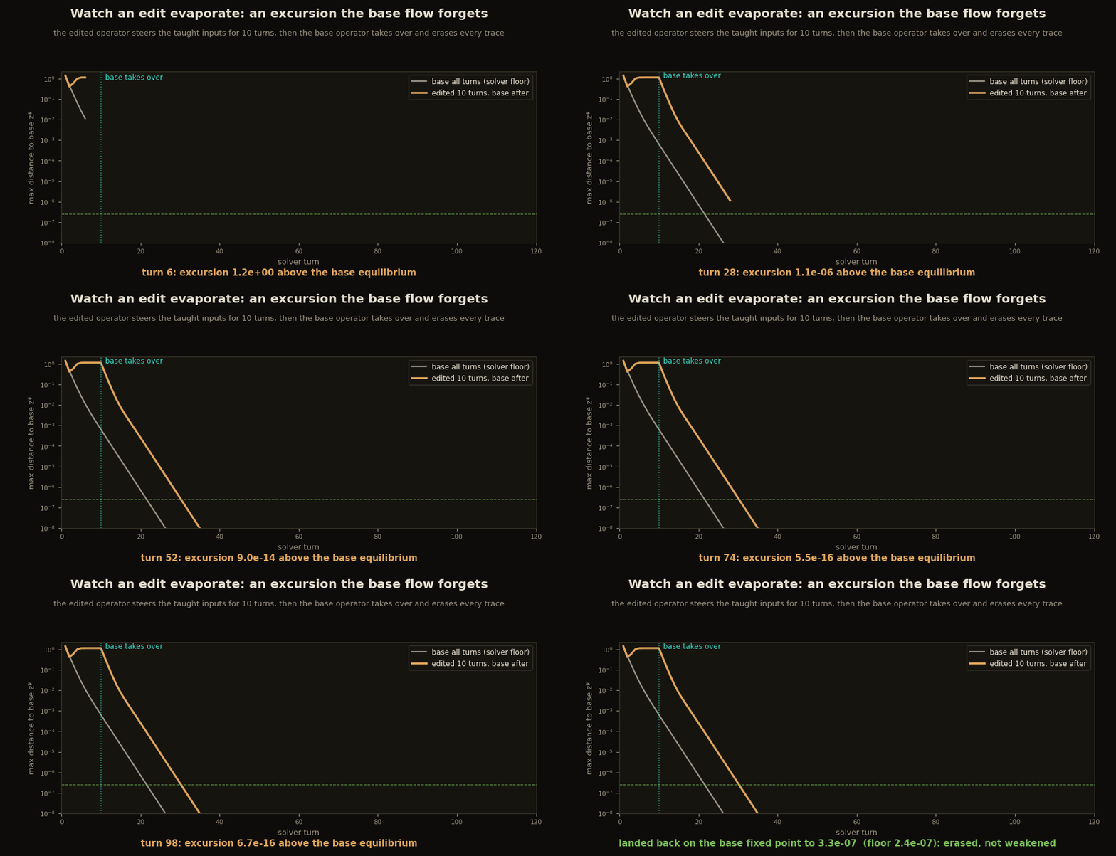
There is a tempting third door: edit a layer. The recursion even seems to allow it, apply the edited operator for the first few turns, then let the base operator take over, the equilibrium version of splicing a modified layer into a stack. What survives at the fixed point?

Xb = Xte[yte == 3]                                         # the taught class
zb_star = model.zstar(Xb)                                  # its base equilibrium
def hybrid(j, total=120):                                  # edited for j turns, base afterwards
    z = jnp.zeros((Xb.shape[0], 32))
    for k in range(total):
        op = edited if k < j else model
        z = (1 - 0.7) * z + 0.7 * op.F(Xb, z)
    return float(jnp.linalg.norm(z - zb_star, axis=1).max())

for j in [0, 3, 10, 30]:
    print(f"edited for first {j:2d} turns:  max dist to base z* = {hybrid(j):.1e}")
# 0: 2.4e-07   3: 3.3e-07   10: 3.3e-07   30: 3.3e-07

Nothing survives. Run the hybrid with the edit steering for the first 3, 10, or 30 turns and the state lands back on the base equilibrium to within 3.3e-07, while the solver’s own noise floor (the run with no edited turns at all) is already 2.4e-07. Not weakened, erased. The reason is the same contraction that makes the model trustworthy: the base flow has one basin with one bottom, so the moment it takes over, it forgets everything the excursion did, geometrically fast. In an equilibrium model there is no such thing as editing a layer, because a fixed point only remembers what acts on it at every depth. The everywhere-edit is not one option among several here; it is the only edit the object admits.

What a stack charges for the same edit#

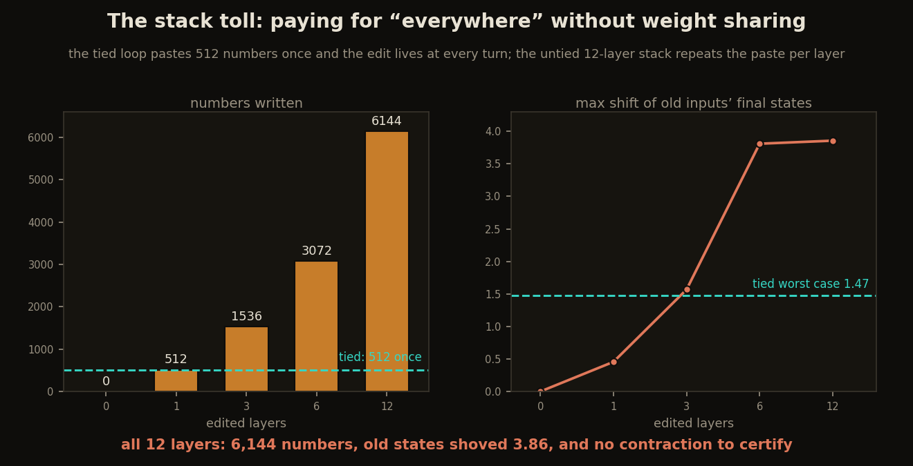
The evaporation result says an edit must exist at every depth to exist at all. The tied network gets that for free; what does it cost when the weights are not shared? The run trains the control, the same architecture with the tying switched off, twelve untied layers, which needs 18,981 parameters to the loop’s 1,733 before anyone edits anything. Reading is cheap everywhere: pasting anchor rows onto the stack’s final state teaches the class at full recall with zero dynamics edits. But putting the class into the dynamics has no single place to go. The paste must be repeated at each layer where the edit should exist.

# the tied loop: one paste, active at every turn
tied_edit_params = anchors.size * 2                        # 512 numbers, once

# the untied stack: the same edit repeated per layer
for j in [0, 1, 3, 6, 12]:
    layers = range(12 - j, 12)
    q, edit_params = stack_edit(stack, states_teach, gamma_frac=0.5, layers=layers)
    dz_old = final_state_shift(q, Xte_old)                 # how far old inputs' final states move
    print(f"edit last {j:2d} layers:  {edit_params:5d} numbers,  max ‖Δz_L‖ old = {dz_old:.2f}")
# 0:    0   0.00      1:  512  0.46      3: 1536  1.57
# 6: 3072  3.81      12: 6144  3.86

Each pasted layer moves old inputs’ final states further, from 0.46 with one layer to 3.86 with all twelve, past the tied edit’s worst case of 1.47. A stack has no single equilibrium operator to audit, so the corresponding object is its end-to-end sensitivity across layers. You pay twelve times for the repeated edit; the tied model needs one paste and one repeatable local audit.

Forgetting splits into two ledgers#

Now run the whole thing backwards. Forget the class we just taught, and the old guarantee returns in full: its knowledge sits in eight appended rows of W and eight columns of A, so slice them off and the operator is restored bit-for-bit.

def forget_taught(edited, M):                              # drop the appended rows
    restored = nnx.clone(edited)
    restored.W = nnx.Param(edited.W.value[:M])
    restored.A = nnx.Param(edited.A.value[:, :M])
    return restored

restored = forget_taught(edited, M=model.W.value.shape[0])
exact = all(bool(jnp.array_equal(restored.__dict__[k].value, model.__dict__[k].value))
            for k in ("W", "A", "Uin", "z0", "C", "cb"))
print("operator restored bit-for-bit:", exact)            # True

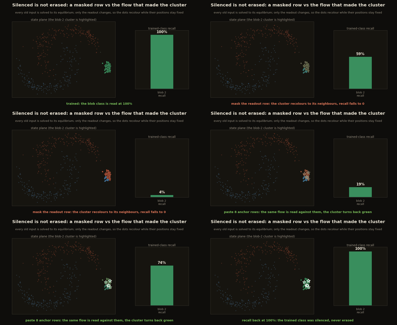
What construction pasted in, deletion removes exactly. But now try to forget a class the network was trained on, and the address book fails for the first time. The trained blob has one readout row, but its knowledge does not live there; gradient descent wove it into the shared bank that every class’s flow runs through. Mask the row and the surface looks like exact unlearning, recall 1.00 to 0.00, the other classes reading literally the same numbers. Yet the flow still carries the class: paste eight anchor rows, the same construction that taught the new class, and the “forgotten” class comes back at 100% recall, no training.

lg = model(Xte_old)
masked = lg.at[:, 2].set(-jnp.inf)                         # mask the trained blob's readout row
print("blob recall:", float((masked[y_old == 2].argmax(-1) == 2).mean()))   # 0.0, silenced

res_anchors = model.zstar(a_region[:8])                    # anchors from the blob's own region
s = alpha * model.kernel(model.zstar(Xte_old), res_anchors).max(-1)
pred = jnp.where(s > masked.max(-1), 2, masked.argmax(-1))
print("resurrected recall:", float((pred[y_old == 2] == 2).mean()))         # 1.0, never erased

That is the boundary: inside a fixed point, what you constructed, you can delete exactly; what you trained, you can only silence. The equilibrium model keeps the exact-unlearning guarantee precisely for the knowledge that lives as rows.

Boundary of the result#

Two rows, two contracts. Readout rows keep every proof from the list network: exact invariance (max |Δ| = 0.0), exact undo, zero gradient steps. Dynamics rows are more powerful: one jnp.concatenate reshapes the operator at every turn, something the stack repeats across twelve layers. In exchange they demand a measurement culture: run local_slope, test multiple starts, re-solve the fixed points, report the drift, and temper the gain when slopes rise. The rows are legible because the state space is low-dimensional and the anchors are settled inputs. True erasure of trained knowledge still means changing the dynamics it is woven into. Editing the network is editing one operator and auditing what that did to everything else.

Deep equilibrium models are from Bai et al. (2019); machine unlearning from Bourtoule et al. (2021); the Yat kernel from Bouhsine (2026). The conceptual companion is Edit One Operator, Edit Every Depth.

@misc{bouhsine2026editafixedpointjaxflaxnnx,
  author       = {Bouhsine, Taha},
  title        = {Editing a Deep Equilibrium Network, in JAX/Flax NNX},
  year         = {2026},
  month        = {jul},
  howpublished = {\url{https://tahabouhsine.com/blog/edit-a-fixed-point-jax-flax-nnx/}},
  note         = {Blog post, Records of the !mmortal Data Scientist}
}