A Network That Is a Fixed Point, in JAX/Flax NNX

The hard part of this network is five lines long and it lives in the backward pass. Everything else is familiar: one shared Flax NNX operator, a loop that runs it until the state stops moving, a linear readout. But you cannot backpropagate through a loop whose length the input chose, so the gradient has to come from the equation rather than the path, which in JAX means jax.custom_vjp and a second fixed-point solve driven by the same iteration as the first. The explainer named that move and never showed it. Here it is, with the operator it differentiates, run on two moons and on maze reachability.

Prefer a notebook? Run the whole thing on Kaggle: the same code, block by block, with the math written out and every figure reproduced from a real run.

One operator, written once#

What is the whole network, in code? A single function that reads its own output. The Yat features score the running state $z$ against a bank of shared prototypes $W$, and the operator mixes those scores, injects the input, and squashes. There is no per-layer weight here: the same $W$, $A$, and $U$ are used on every turn.

import jax, jax.numpy as jnp
from flax import nnx

class YatDEQ(nnx.Module):
    """One shared Yat operator F(z; x) = tanh(A · φ_W(z) + U x + z0), reused at every depth."""
    def __init__(self, d_in, d, m, ncls, *, rngs):
        k = rngs.params()
        self.W   = nnx.Param(jax.random.normal(k, (m, d)) * 0.6)          # m shared prototypes in state space
        self.A   = nnx.Param(jax.random.normal(k, (d, m)) * (0.5 / m ** 0.5))  # small -> encourages contraction
        self.Uin = nnx.Param(jax.random.normal(k, (d, d_in)) * 0.5)       # input injection, every turn
        self.z0  = nnx.Param(jnp.zeros((d,)))
        self.b   = nnx.Param(jnp.full((), 0.5)); self.eps = nnx.Param(jnp.full((), 1.0))
        self.C   = nnx.Param(jax.random.normal(k, (ncls, d)) * 0.5)       # linear readout on z*
        self.cb  = nnx.Param(jnp.zeros((ncls,)))

    def phi(self, z):                                                     # φ_W(z): state-to-prototype similarities
        b, eps = jax.nn.softplus(self.b.value), jax.nn.softplus(self.eps.value)
        dot = z @ self.W.value.T
        d2  = (z ** 2).sum(-1, keepdims=True) + (self.W.value ** 2).sum(-1) - 2 * dot
        return (dot + b) ** 2 / (d2 + eps)

    def F(self, z, x):                                                    # one application of the operator
        return jnp.tanh(self.phi(z) @ self.A.value.T + x @ self.Uin.value.T + self.z0.value)

That is the entire network, at any depth. An ordinary deep net would hold a fresh W_ℓ and A_ℓ per layer; here F is a method, and depth is just how many times you call it. For two moons the state lives in 32 dimensions, there are 24 shared prototypes, and the whole thing is 1700 numbers, the same count whether the solver turns six times or sixty.

Solving the equation, not marching a stack#

How do you run a network with no fixed depth? You iterate the operator until its output stops changing. The state starts at zero and each turn nudges it toward the fixed point; a little damping ($\beta = 0.7$) keeps the iteration stable. When the step size falls below a tolerance, the state has arrived, and that resting point $z^\*$ is the answer.

def solve(F, x, z0, iters=120, beta=0.7):
    """Damped Picard: z_{k+1} = (1-β) z_k + β F(z_k). Returns z* and the residual trace."""
    def step(z, _):
        zn = (1 - beta) * z + beta * F(z, x)
        return zn, jnp.max(jnp.linalg.norm(zn - z, axis=-1))     # per-step max residual
    z_star, resid = jax.lax.scan(step, z0, None, length=iters)
    return z_star, resid

One number tells you whether that loop terminated or merely ran out of budget: the size of the last step. Drop one input in, iterate, and watch it collapse while the state rolls into its resting point.

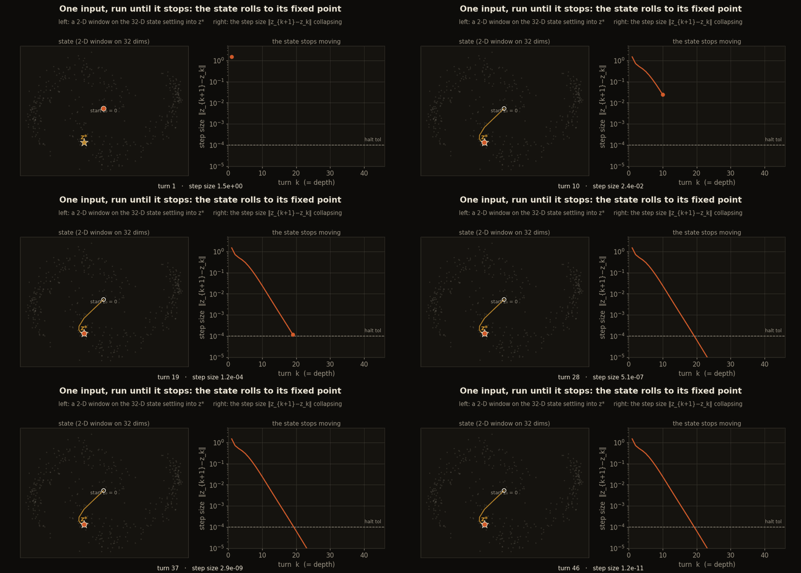
The straight-line collapse on the log axis shows geometric convergence along this trajectory: each turn shrinks the step by a near-constant factor. Across the test set the residual reaches about $4\times10^{-7}$, so the solver meets its stopping rule rather than merely running out of iterations.

Testing local stability and initialization sensitivity#

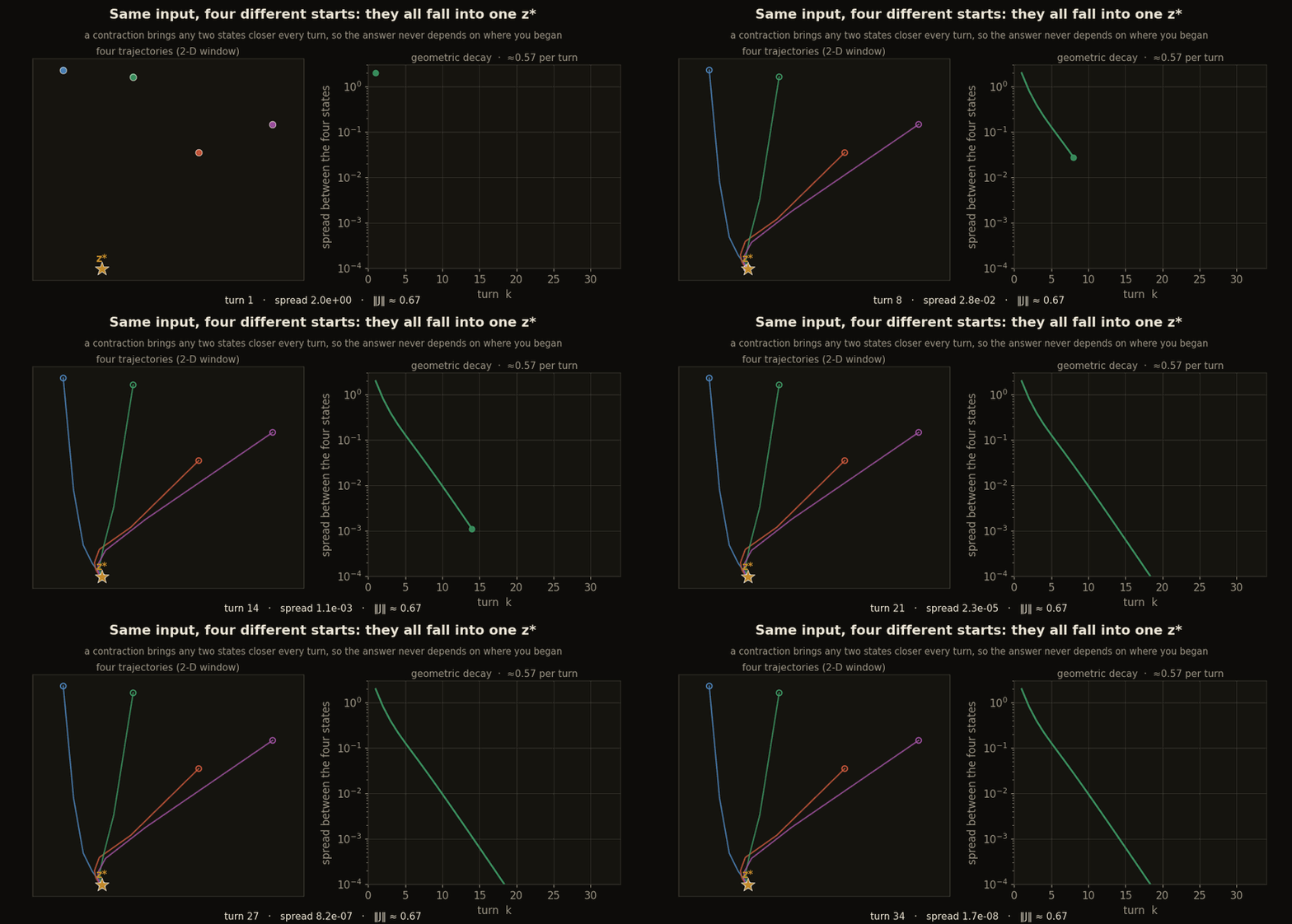
A global contraction satisfies $\lVert F(z)-F(z')\rVert\leq\rho\lVert z-z'\rVert$ for every pair in a stated domain and some $\rho<1$. Banach’s theorem would then guarantee one fixed point reached from every start in that domain. The calculation below is narrower: it estimates the top singular value of $J_F$ at each observed equilibrium. That measures local stability around those points; it does not take the supremum over state space required for a global certificate.

def spectral_norm(model, x, z_star, key, iters=6):
    """‖J_F‖₂ at z* by power iteration on JᵀJ (differentiable in params; direction detached)."""
    fz = lambda zz: model.F(zz, x)
    v = jax.random.normal(key, z_star.shape)
    v = v / (jnp.linalg.norm(v, axis=-1, keepdims=True) + 1e-9)
    for _ in range(iters):
        Jv = jax.jvp(fz, (z_star,), (v,))[1]                    # J v
        JtJv = jax.vjp(fz, z_star)[1](Jv)[0]                    # Jᵀ (J v)
        v = jax.lax.stop_gradient(JtJv / (jnp.linalg.norm(JtJv, axis=-1, keepdims=True) + 1e-9))
    return jnp.linalg.norm(jax.jvp(fz, (z_star,), (v,))[1], axis=-1)   # ≈ ‖J‖₂ per sample

Nothing forces the raw operator to be locally stable, so the loss penalizes $\lVert J_F(z^*;x)\rVert$ at training equilibria. After training the measured slope averages 0.66 and tops out at 0.92 across the test set. A second test fixes one input and starts the solver from four widely separated states; all four tested trajectories reach the same observed $z^*$.

The penalty rides alongside the cross-entropy in the loss, evaluated at the equilibrium (detached, so the contraction term shapes the operator without fighting the readout gradient).

import optax

def loss_fn(model, x, y, key):
    z_star = deq(model, x)                                       # forward fixed-point solve (below)
    logits = z_star @ model.C.value.T + model.cb.value
    ce = optax.softmax_cross_entropy_with_integer_labels(logits, y).mean()
    sigma = spectral_norm(model, x, jax.lax.stop_gradient(z_star), key)
    contract = 3.0 * jnp.mean(jax.nn.relu(sigma - 0.7) ** 2)     # 0 once ‖J‖₂ < target
    return ce + contract

Trained through what, exactly: implicit differentiation#

The forward pass is “iterate until it stops”: fourteen turns for one input, sixty-five for another. Unrolling whatever it happened to take, storing every intermediate state to backpropagate through, would cost memory that grows with the turn count, and it would betray the framing: we said the answer was the solution of an equation, not the path to it. So do not differentiate the path. Differentiate the equation.

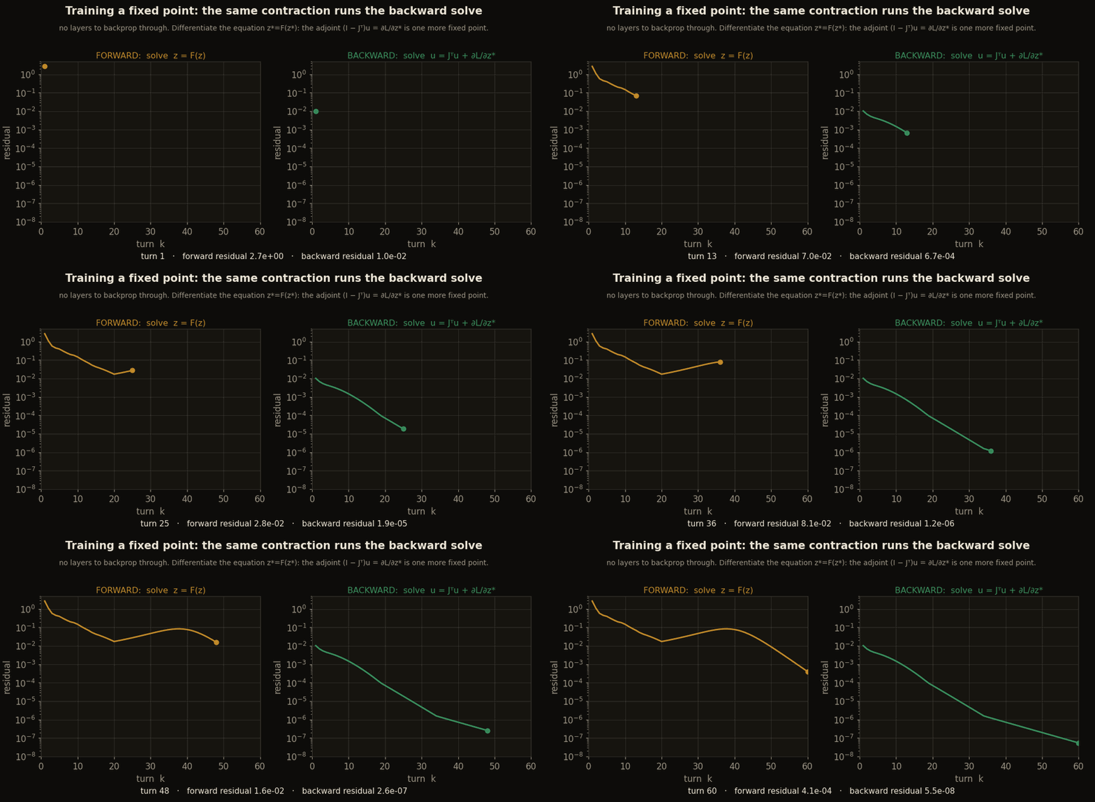
The fixed point satisfies $z^\* = F(z^\*; x)$, an identity. Differentiating it makes the chain rule fold into itself, $dz^\* = J_F\,dz^\* + \partial_\theta F$, and the gradient becomes one linear solve in the Jacobian: the adjoint $(I - J_F^\top)\,u = \partial\mathcal{L}/\partial z^\*$. And $u = J_F^\top u + \partial\mathcal{L}/\partial z^\*$ is itself a fixed-point equation, so the same damped iteration that ran the forward solve runs the backward one, at constant memory no matter how many forward turns there were. We wire this into JAX with a custom vector-Jacobian product.

from functools import partial

@partial(jax.custom_vjp, nondiff_argnums=())
def deq(model, x):
    z0 = jnp.zeros((x.shape[0], model.z0.value.shape[0]))
    z_star, _ = solve(model.F, x, z0)
    return z_star

def deq_fwd(model, x):
    z0 = jnp.zeros((x.shape[0], model.z0.value.shape[0]))
    z_star, _ = solve(model.F, x, z0)
    return z_star, (model, x, z_star)

def deq_bwd(res, g):
    model, x, z_star = res
    # z* = F(z*), so the cotangent obeys (I − Jᵀ) u = g  ->  u = Jᵀu + g, another fixed point.
    _, vjp_z = jax.vjp(lambda z: model.F(z, x), z_star)          # Jᵀ · (·)
    u, _ = solve(lambda u, _: vjp_z(u)[0] + g, None, jnp.zeros_like(g))   # SAME iteration, backward
    # push u back through the params/input, no unrolled solver in sight
    _, vjp_px = jax.vjp(lambda mm, xx: mm.F(z_star, xx), model, x)
    g_model, g_x = vjp_px(u)
    return g_model, g_x

deq.defvjp(deq_fwd, deq_bwd)

The elegance is that the two solves are the same solve. The contraction that made the forward iteration converge ($\lVert J_F\rVert < 1$) makes the backward one converge too, by the identical Banach argument, because $J_F^\top$ has the same spectral norm as $J_F$. Run both from the trained operator and their residuals fall on the same kind of geometric line.

Depth becomes a dial the input turns#

If depth is iteration count, how much of it does any input actually need? Apply the operator a chosen number of times across the whole input plane and color each point with the decision it would give if it stopped there. For the first several turns the boundary is still forming; then it snaps into place and freezes.

def boundary_at_depth(model, grid, k):
    z = jnp.zeros((grid.shape[0], model.z0.value.shape[0]))
    for _ in range(k):                                          # k turns of the shared operator
        z = 0.3 * z + 0.7 * model.F(z, grid)
    return jax.nn.softmax(z @ model.C.value.T + model.cb.value, -1)[:, 1]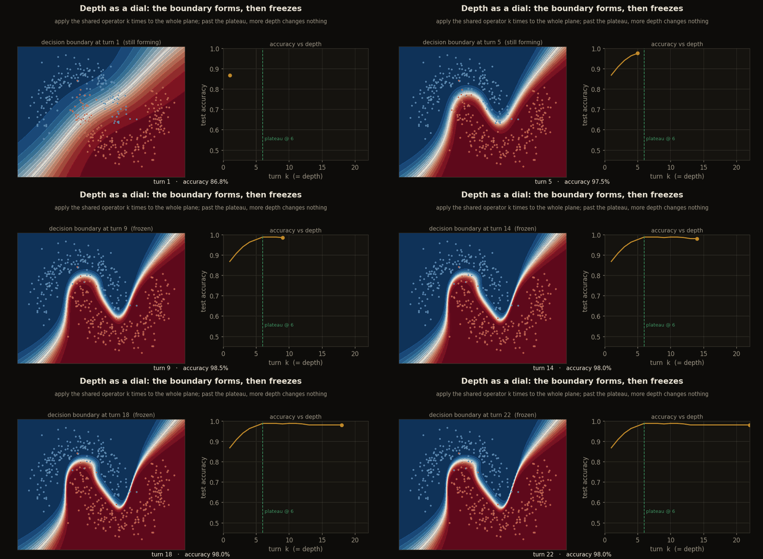

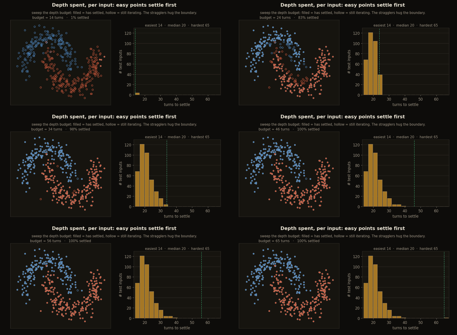
The classification is settled by about the sixth turn and never changes afterward, so the halting rule “stop when the answer stops moving” is safe. And the number of turns is not a constant: easy inputs deep inside a class settle fast, hard inputs on the boundary take longer.

def iters_to_settle(model, x, tol=1e-4, maxk=120):
    z = jnp.zeros((x.shape[0], model.z0.value.shape[0]))
    ks = jnp.full((x.shape[0],), maxk)
    for k in range(maxk):
        zn = 0.3 * z + 0.7 * model.F(z, x)
        r = jnp.linalg.norm(zn - z, axis=-1)
        ks = jnp.where((r < tol) & (ks == maxk), k + 1, ks)     # first turn each input settles
        z = zn
    return ks                                                   # per-input adaptive depth

Sweep the budget and the confident interiors fill in first; the stragglers are precisely the ambiguous points hugging the boundary. The real spread runs from 14 turns for the easiest input to a median of 20 and 65 for the single hardest.

Why go deep at all: a maze that makes you earn it#

Two moons settled in six turns, so why build a machine that can go a thousand? Because some problems make depth the point. Grid reachability spreads one ring per step out from a goal, so a cell forty hops away genuinely cannot be decided in fewer than forty turns. We share one Yat operator across all of them, reading each cell’s five-cell neighbourhood and masked by the walls: a weight-tied recurrent convolution.

def patch(z):                                                   # the 5-cell neighborhood, self + 4 neighbors
    return jnp.concatenate([z, shift(z, 1, 0), shift(z, -1, 0),
                            shift(z, 0, 1), shift(z, 0, -1)], -1)

def maze_F(p, z, x, free):                                       # one turn of the shared grid operator
    pt = patch(z)
    dot = pt @ p['W'].T
    d2  = (pt ** 2).sum(-1, keepdims=True) + (p['W'] ** 2).sum(-1) - 2 * dot
    phi = (dot + p['b']) ** 2 / (d2 + p['eps'])                  # Yat feature on the neighborhood
    return jnp.tanh(phi @ p['A'].T + x @ p['Uin'].T + p['z0']) * free   # walls carry nothing

We train this only on small $11\times11$ grids, unrolled for 30 turns, so no front it ever followed traveled more than thirty steps. Then we hand it a $27\times27$ maze whose front must travel forty cells and more, into territory no training run reached. Everything about generalization says it should fall apart. It does not: it floods right past the training line and solves the mazes to 99.5% of cells, as long as you let it iterate long enough for the front to arrive.

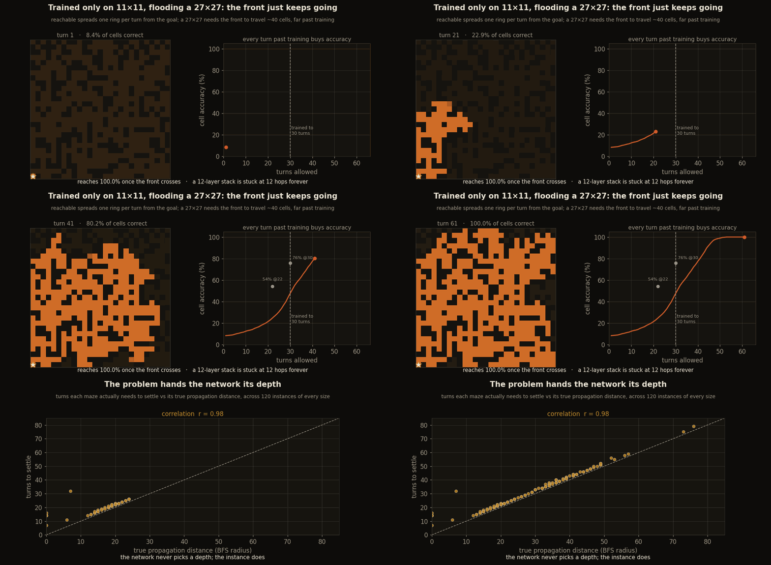
The scatter closes the circle with the adaptive-depth story: the turns each maze needs track its true propagation distance almost perfectly, $r = 0.98$. The network never picks a depth. The problem hands it one.

What the code buys#

The whole two-moons network, at any depth, is 1700 parameters, one operator $(W, A, U, C)$ reused for every turn, and it still reaches 98.2% on the interleaving moons. The maze operator is smaller still and solves grids far larger than any it trained on. The two ideas that made all of it work are short: solve is a damped Picard iteration, and deq_bwd is the same iteration run backward, the implicit function theorem in five lines. No stack of activations is ever stored, because there is no stack. The network is an equation, and the code solves it, forward and backward, the same way.

# put together: train the fixed point end to end
model = YatDEQ(d_in=2, d=32, m=24, ncls=2, rngs=nnx.Rngs(0))
optimizer = nnx.Optimizer(model, optax.adam(3e-3))

@nnx.jit
def train_step(model, optimizer, x, y, key):
    grads = nnx.grad(loss_fn)(model, x, y, key)                 # flows through deq_bwd (implicit diff)
    optimizer.update(grads)

# ... it lands at 98.2% test on two moons, ‖J‖ mean 0.66 / max 0.92, residual ~4e-7 ...

The deep-equilibrium framing is from Bai, Kolter, and Koltun (2019); the contraction/monotone-operator view from Winston and Kolter (2020); Jacobian regularization for stability from Bai, Koltun, and Kolter (2021); the Yat kernel from Bouhsine (2026). The conceptual companion is Your Network Is a Stack of Layers. It Could Be a Fixed Point.

@misc{bouhsine2026yournetworkisafixedpointjaxflaxnnx,
  author       = {Bouhsine, Taha},
  title        = {A Network That Is a Fixed Point, in JAX/Flax NNX},
  year         = {2026},
  month        = {jul},
  howpublished = {\url{https://tahabouhsine.com/blog/your-network-is-a-fixed-point-jax-flax-nnx/}},
  note         = {Blog post, Records of the !mmortal Data Scientist}
}