Building the Second Layer by Hand, in JAX/Flax NNX
#ml#kernels#interpretability#prototypes#computer-vision#construction#depth#jax#flax#nnx#yat#deep-learning
Part 3 of 9The Prototype Network
- 1Your Network Is a List of Pictures. You Can Edit It.
- 2How Much of a Fashion-MNIST Network Can You Build by Hand?
- 3How Far Down Can You Build?this post's explainer
- 4When 80% Should Mean 80%
- 5The White-Box Survival Model on Trial
- 6Your Network Is a Stack of Layers. It Could Be a Fixed Point.
- 7Edit One Operator, Edit Every Depth
- 8One Kernel Family, Fitted Two Ways
- 9How Many Random Neurons Buy a Trained One?
The second feature layer is four lines of np.minimum. That is not a summary of it, that is the layer: junctions, continuations, bends and stripes are each one pointwise AND over the hand-built first layer’s maps, and the classifier sitting on top is the same Flax NNX module of placed k-means prototypes as before, with no training loop anywhere in the post. The explainer reports what a century of vision science buys when you spend it this way: 82.9% for both layers, against 83.3% for one. The code is short enough to see why.
Prefer a notebook? Run the whole thing on Kaggle: the same code, block by block, with the math written out and every figure reproduced from a real run.
What layer 2 is made of
What can a second layer even say? Only things about the first. Layer 1’s whole vocabulary is seven words per cell, six oriented-edge energies and a corner, so layer 2 has to be sentences that relate those words. The cheapest faithful AND between two non-negative energies is their minimum, and four kinds of sentence fall out of it: a junction (two orientations in one cell), a continuation (one orientation one cell along its own direction), a bend (a continuation that arrives rotated a step), and a stripe (a parallel echo two cells across). Layer 1 comes in unchanged from the last companion, mean-pooled to a 14-by-14 cell grid so layer 2 has neighbours to reach into.
import numpy as np, math
from scipy.ndimage import convolve

NB, NCH, CELL = 6, 7, 14                                  # 6 orientations + corner, on a 14x14 cell grid
CENTERS = np.linspace(0, np.pi, NB, endpoint=False)
CONTOUR = [(-math.sin(a), math.cos(a)) for a in CENTERS]  # unit step along each edge's own direction
SX = np.array([[-1, 0, 1], [-2, 0, 2], [-1, 0, 1]], 'float32'); SY = SX.T

def channel_maps(X):                                      # layer 1, verbatim from the last post
    gx = np.stack([convolve(im, SX, mode='nearest') for im in X])
    gy = np.stack([convolve(im, SY, mode='nearest') for im in X])
    mag = np.sqrt(gx ** 2 + gy ** 2) + 1e-6
    ang = np.arctan2(gy, gx) % np.pi
    out = [np.clip(1 - np.abs(((ang - CENTERS[b] + np.pi / 2) % np.pi) - np.pi / 2) / (np.pi / NB), 0, 1) * mag
           for b in range(NB)]
    out.append(np.abs(gx) * np.abs(gy))                   # corner
    return np.stack(out, 1)                               # [n, 7, 28, 28]

def cells(maps):                                          # 2x2 mean-pool to the 14x14 cell grid
    n = len(maps)
    return maps.reshape(n, NCH, CELL, 2, CELL, 2).mean((3, 5))
A junction is the whole idea in one picture: take the map of one orientation and the map of another, and keep only where both fire. That pointwise minimum is a new detector, computed from layer 1 the same way layer 1 was computed from pixels, with nothing fit.
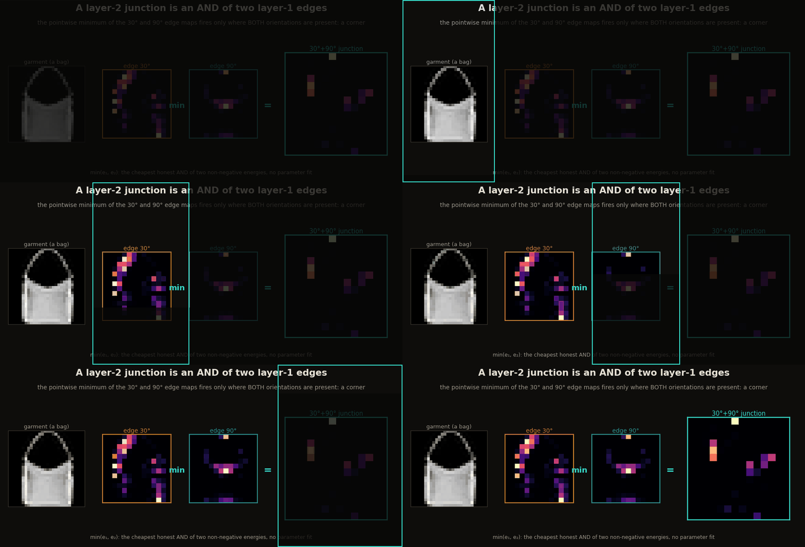
np.minimum(e1, e2), the cheapest faithful AND of two non-negative energies, no parameter fit. The animation reveals the garment, the two edge maps, and their minimum in computational order.The four lines that are the layer
The whole second layer is those four sentences, written once and evaluated on the cell grid. A junction is a min of two orientations in place; a continuation is a min of an orientation with itself shifted one cell along its contour; a bend swaps the shifted partner for the neighbouring orientation; a stripe reaches across the edge instead of along it. The shift is bilinear, so a contour that runs at 30° is followed at 30°, not snapped to the pixel grid.
def shift_frac(A, dy, dx):                                # sample A at (y+dy, x+dx), bilinear
    y0, x0 = math.floor(dy), math.floor(dx); fy, fx = dy - y0, dx - x0
    def sh(a, iy, ix):
        out = np.zeros_like(a); h, w = a.shape[-2:]
        ys, xs = max(0, -iy), max(0, -ix); ye, xe = min(h, h - iy), min(w, w - ix)
        if ye > ys and xe > xs: out[..., ys:ye, xs:xe] = a[..., ys + iy:ye + iy, xs + ix:xe + ix]
        return out
    return ((1 - fy) * (1 - fx) * sh(A, y0, x0) + (1 - fy) * fx * sh(A, y0, x0 + 1)
            + fy * (1 - fx) * sh(A, y0 + 1, x0) + fy * fx * sh(A, y0 + 1, x0 + 1))

def l2_maps(C):                                           # [n, 33, 14, 14]: the named layer-2 vocabulary
    E = C[:, :NB]; out = []
    for b1 in range(NB):                                  # 15 junctions
        for b2 in range(b1 + 1, NB):
            out.append(np.minimum(E[:, b1], E[:, b2]))
    for b in range(NB):                                   # 6 continuations
        dx, dy = CONTOUR[b]
        out.append(np.minimum(E[:, b], shift_frac(E[:, b], dy, dx)))
    for b in range(NB):                                   # 6 bends: the continuation arrives rotated a step
        dx, dy = CONTOUR[b]
        nb = np.maximum(shift_frac(E[:, (b + 1) % NB], dy, dx), shift_frac(E[:, (b - 1) % NB], dy, dx))
        out.append(np.minimum(E[:, b], nb))
    for b in range(NB):                                   # 6 stripes: a parallel echo two cells across
        gdx, gdy = math.cos(CENTERS[b]), math.sin(CENTERS[b])
        echo = np.maximum(shift_frac(E[:, b], gdy * 2, gdx * 2), shift_frac(E[:, b], -gdy * 2, -gdx * 2))
        out.append(np.minimum(E[:, b], echo))
    return np.stack(out, 1)
Fifteen junction pairs, six continuations, six bends, six stripes: 33 named detectors, each one sentence long. Re-pooled over a 4-by-4 grid that is 33 × 16 = 528 new dimensions, and every one is still nameable (“a 30°+90° junction in the top-right region”). None of it was trained.
The head is the same placed module
What classifies these features? The exact head from the first two companions, unchanged. The constructed Yat head is a Flax NNX module whose variables are placed, not learned: W holds k-means centroids of the training features, A is a one-hot table routing each prototype’s vote to its class, and the forward pass is the Yat kernel against every prototype, then the per-class maximum, then an argmax. It slots onto layer-2 features without a line changing, which is the whole reason the comparison is clean: depth changed the representation and nothing else.
from flax import nnx
import jax, jax.numpy as jnp

class YatHead(nnx.Module):
    """Placed prototypes W (k-means centroids), one-hot votes A, nearest-prototype vote."""
    def __init__(self, W, vote, b=0.5, eps=1.0):
        self.W = nnx.Variable(jnp.asarray(W))                        # [K, D] prototypes, D = 343 or 528 or 871
        self.A = nnx.Variable(jax.nn.one_hot(jnp.asarray(vote), 10))
        self.b, self.eps = b, eps

    def __call__(self, z):                                          # z: [N, D] features
        dot = z @ self.W.value.T
        d2 = (z ** 2).sum(1, keepdims=True) + (self.W.value ** 2).sum(1) - 2 * dot
        ker = (dot + self.b) ** 2 / (d2 + self.eps)                 # the Yat kernel
        scores = jnp.where(self.A.value.T[None].astype(bool), ker[:, None, :], -jnp.inf).max(-1)
        return scores.argmax(-1)
There is still no nnx.Param in it. nnx.Variable is the right type for state an optimizer would never touch, and the whole depth experiment reuses this one module three times: on layer 1 alone, on layer 2 alone, and on the two concatenated.
The flat rung
Now assemble it, which is just extract, z-score, place prototypes, set the softening ε from the data’s own scale, and read the argmax. Doing that for layer 1 alone reproduces the number the series has carried since the first hand-built post.
from sklearn.cluster import KMeans

def build_and_eval(Ftr_raw, Fte_raw, ytr, yte, per=20):
    mu, sd = Ftr_raw.mean(0), Ftr_raw.std(0) + 1e-6
    Ftr, Fte = (Ftr_raw - mu) / sd, (Fte_raw - mu) / sd            # z-score into the head's space
    W, vote = [], []
    for c in range(10):
        W += list(KMeans(per, n_init=2, random_state=0).fit(Ftr[ytr == c][:2500]).cluster_centers_)
        vote += [c] * per
    W = np.array(W, 'float32'); vote = np.array(vote)
    d2 = (Fte ** 2).sum(1, keepdims=True) + (W ** 2).sum(1) - 2 * Fte @ W.T
    eps = float(np.median(d2) * 0.1)                                # placed, like everything else
    head = YatHead(W, vote, b=0.5, eps=eps)
    return 100 * (np.asarray(head(jnp.asarray(Fte))) == yte).mean()

# layer 1 alone (343 named dims) -> 83.3%
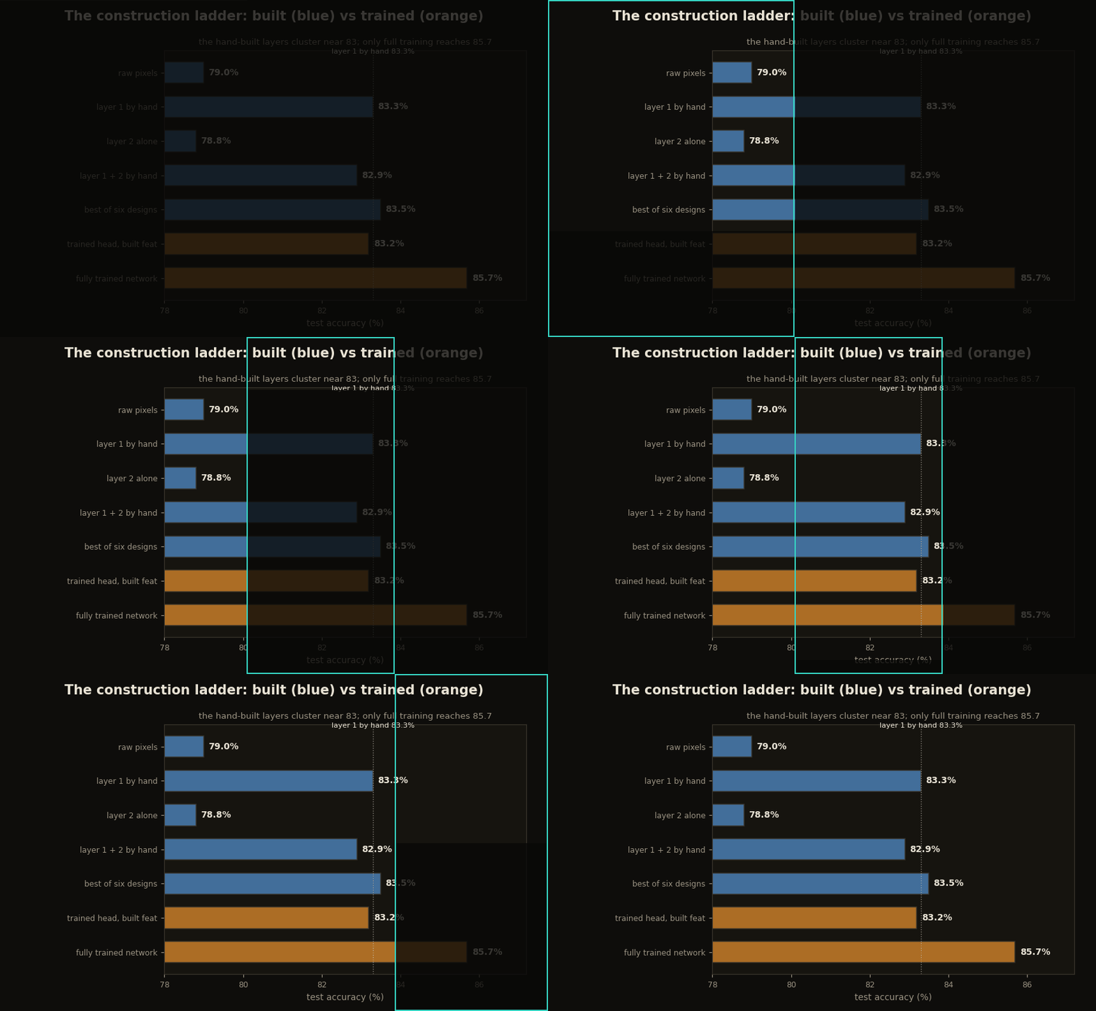
It prints 83.3%. The obvious next move is to concatenate the 528 layer-2 dimensions onto the 343 and run the same head. That is the whole experiment, and the whole disappointment.
Fc_tr = np.concatenate([F1tr, F2tr], 1)                            # 343 + 528 = 871 named dims
Fc_te = np.concatenate([F1te, F2te], 1)
acc = build_and_eval(Fc_tr, Fc_te, ytr, yte)                       # -> 82.9%
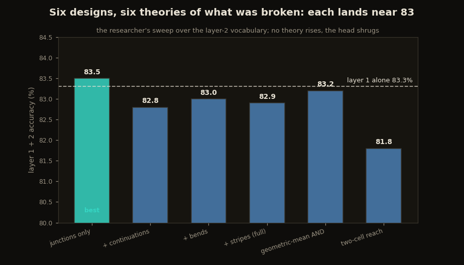
It prints 82.9%, a drop of 0.4 points from a layer of century-old vision science. Iterating as we would on any model, with each redesign expressing a theory of what broke, does not help: junctions alone score 83.5% (the best of six designs), and the rest land at 82.8, 83.0, 82.9, and, for a geometric-mean AND and a two-cell reach, 83.2 and 81.8. Six theories, six refutations by a few tenths.
The detectors are real, and that is the trap
Flat rung, so the detectors must be junk? The code says otherwise. Throw away all 343 edge dimensions and classify from layer 2 alone, nothing but junctions, continuations, bends and stripes, and it reaches 78.8%, within a fifth of a point of the raw-pixel network’s 79.0. Detectors that never see a raw edge recover almost the entire baseline: they carry genuine class signal.
build_and_eval(F2tr, F2te, ytr, yte) # layer 2 ALONE -> 78.8%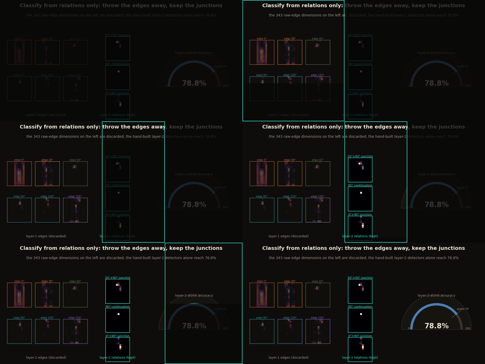
So why does adding them to layer 1 do nothing? Because they are synonyms. Every layer-2 value is a fixed function of layer-1 values, and a min of two edges says nothing the pair of edges had not already said. The kernel head reads whole vectors, so it was already comparing garments on those coordinates jointly; rewriting the same information in a richer vocabulary gives it nothing new to vote with. You can see the redundancy directly: correlate each layer-2 detector with the layer-1 channels it is built from, and the structure is not noise, it is the detector spelling out its own recipe.
L1 = Ctr.mean((2, 3))                                              # per-channel layer-1 energy [n, 7]
L2 = l2_maps(Ctr).mean((2, 3))                                    # per-detector layer-2 energy [n, 33]
L1z = (L1 - L1.mean(0)) / (L1.std(0) + 1e-9)
L2z = (L2 - L2.mean(0)) / (L2.std(0) + 1e-9)
corr = (L2z.T @ L1z) / len(L1)                                    # each row: a layer-2 dim's edge recipe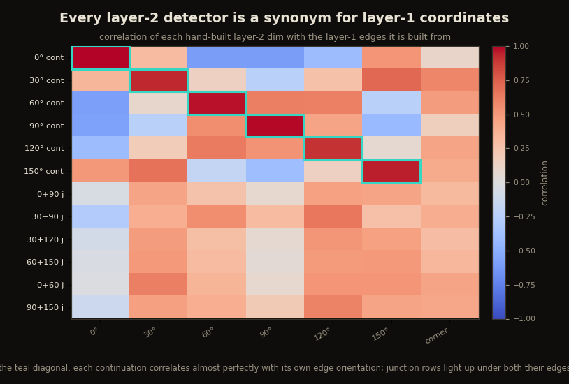
Counting the wall
Maybe the fix is just the right 33 sentences. That objection is correct, and it is the whole finding, once you count what “right” would cost. A pairwise layer-2 type is two channels at a relative cell offset, and within a one-cell neighbourhood there are 224 nameable types; three-way combinations, the kind a trained CNN routinely represents, run to roughly 4,630 before you have even chosen pooling or the form of the AND. We hand-picked 33 of the 224 using the best prior our species has about early vision, and moved the needle +0.2 at best.
same = NCH * (NCH + 1) // 2                                       # offset (0,0), unordered incl. self-pairs
shifted = NCH * NCH * 8 // 2                                      # 8 nonzero offsets, halved by symmetry
pairs_possible = same + shifted                                  # 224
triples_possible = (NCH ** 3) * (9 ** 2) // 6                     # ~4,630 three-way types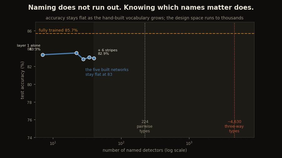
What this measures
Run this script and the ladder reads the same thing the explainer argues: construction is not a rival to training that fell 2.4 points short, it is a measurement instrument. It reports, layer by layer, how much of a network is generic structure a person could write (all of the classifier, all of layer 1, 83.3 of the 85.7 points) and how much is data-selected combination (the rest). At layer 1, naming and helping coincided, so human priors could curate the vocabulary completely. One layer up they come apart: picking the few combinations that add signal, jointly, against what the layer below already provides, is a search over thousands of coupled candidates with the data as judge. The code names that search plainly. It is called training.
Oriented-edge first stages are from Hubel and Wiesel (1962); the edges-then-tokens grammar is Marr’s primal sketch (Vision, 1982); the layer-1 detectors follow the HOG lineage of Dalal and Triggs (2005); Fashion-MNIST from Xiao et al. (2017); the Yat kernel from Bouhsine (2026). The conceptual companion is How Far Down Can You Build?.
Cite as
Bouhsine, T. (). Building the Second Layer by Hand, in JAX/Flax NNX. Records of the !mmortal Data Scientist. https://tahabouhsine.com/blog/depth-by-construction-jax-flax-nnx/
BibTeX
@misc{bouhsine2026depthbyconstructionjaxflaxnnx,
  author       = {Bouhsine, Taha},
  title        = {Building the Second Layer by Hand, in JAX/Flax NNX},
  year         = {2026},
  month        = {jul},
  howpublished = {\url{https://tahabouhsine.com/blog/depth-by-construction-jax-flax-nnx/}},
  note         = {Blog post, Records of the !mmortal Data Scientist}
}References
- (1962). Receptive Fields, Binocular Interaction and Functional Architecture in the Cat's Visual Cortex. The Journal of Physiology 160, 106–154.
- (1982). Vision: A Computational Investigation into the Human Representation and Processing of Visual Information. W. H. Freeman.
- (2005). Histograms of Oriented Gradients for Human Detection. CVPR 2005.
- (2017). Fashion-MNIST: a Novel Image Dataset for Benchmarking Machine Learning Algorithms. arXiv:1708.07747
- (2026). A Universal Reproducing Kernel Hilbert Space from Polynomial Alignment and IMQ Distance. arXiv:2605.03262