A Kernel's Price List, in JAX
#ml#kernels#rkhs#spectral-analysis#jax#sobolev#fourier#smoothness#implementation
Part 3 of 4Weights in Kernel Space
The explainer calls a kernel a price list: each spectral mode has an eigenvalue, and a function pays the squared size of that mode divided by the eigenvalue. This companion computes the bill without smuggling in a spectrum that the kernel does not have.
The safe direction is spectrum first. Choose nonnegative Fourier coefficients, obtain a positive-definite periodic kernel automatically, and then inspect which functions its RKHS can afford.
The domain is part of the kernel
Work on the circle with uniform measure. A translation-invariant kernel has a Fourier expansion
and it is positive definite exactly when . For a real even kernel, .
This is where a tempting shortcut fails: sample a nonperiodic radial function on a finite interval, join the endpoints implicitly with an FFT, and call the coefficients eigenvalues. That operation analyzes the periodic extension created by the sampling grid. If that extension is not positive definite, some coefficients become negative and the resulting “RKHS norm” is not an RKHS norm.
Build the valid object in the other direction:
import jax
import jax.numpy as jnp

jax.config.update("jax_enable_x64", True)

N = 2048
freq = jnp.fft.rfftfreq(N, d=1 / N)       # 0, 1, ..., N/2

def positive_spectrum(kind, *, s=1.0, sigma=0.18, rho=0.88):
    m = freq
    if kind == "sobolev":
        return (1.0 + m**2) ** (-s)        # polynomial tail
    if kind == "heat":
        return jnp.exp(-0.5 * sigma**2 * m**2)  # Gaussian tail
    if kind == "poisson":
        return rho**m                     # exponential tail
    raise ValueError(kind)

def kernel_samples(lam):
    # irfft constructs the real periodic kernel represented by lam.
    return jnp.fft.irfft(lam, n=N) * N

spectra = {name: positive_spectrum(name)
           for name in ("sobolev", "heat", "poisson")}

for name, lam in spectra.items():
    assert bool(jnp.all(lam >= 0)), name
    print(name, float(lam[8]), float(lam[32]))
The assertion is not a cosmetic numerical check. Nonnegative Fourier coefficients are the positive-definiteness condition for this periodic translation-invariant construction.
Three valid price lists
The examples isolate three decay classes:
| family | eigenvalues | high-frequency price |
|---|---|---|
| periodic Sobolev | polynomial | |
| heat kernel | Gaussian | |
| Poisson kernel | exponential |
All three are positive-definite kernels on the circle. Their native spaces differ because their tails differ. The Sobolev spectrum leaves high frequencies expensive but attainable at a polynomial rate. The Poisson and heat spectra charge exponentially and Gaussianly increasing prices.
Compute a bill, then ask whether it converges
For Fourier coefficients , the formal RKHS norm is
On a finite grid we can compute only a partial sum. A partial sum is a measurement at resolution , not a proof that the infinite series converges. The useful experiment is therefore a convergence curve over increasing cutoffs.
x = 2 * jnp.pi * jnp.arange(N) / N
tent = 1.0 - jnp.abs((x - jnp.pi) / jnp.pi)  # continuous, one sharp corner
fhat = jnp.fft.rfft(tent) / N

def partial_bills(fhat, lam, cutoffs=(8, 16, 32, 64, 128, 256, 512)):
    terms = jnp.abs(fhat) ** 2 / jnp.maximum(lam, 1e-300)
    return jnp.array([jnp.sum(terms[:M + 1]) for M in cutoffs])

for name, lam in spectra.items():
    print(name, partial_bills(fhat, lam))
A tent has Fourier coefficients of order . With the first-order Sobolev spectrum, its norm terms scale like , so the partial bills converge. With a Poisson spectrum they scale like and diverge; with the heat spectrum they grow faster still.
The code and the asymptotics now test each other. If the numerical partial sums disagree with the predicted tail, the implementation is wrong or the grid has not reached the asymptotic regime.
Finite precision is not infinity
Exponentially small eigenvalues reach floating-point limits quickly. Clipping them avoids division by zero, but clipping also changes the kernel and its norm. Report both the cutoff and the smallest eigenvalue used:
def audited_partial_bill(fhat, lam, M, floor=1e-280):
    used = lam[:M + 1]
    if bool(jnp.any(used <= floor)):
        return {"M": M, "status": "precision limit", "min_lambda": float(used.min())}
    bill = jnp.sum(jnp.abs(fhat[:M + 1])**2 / used)
    return {"M": M, "status": "measured", "bill": float(bill),
            "min_lambda": float(used.min())}
“The bill exceeded 15 by mode 90” is a plotting threshold. “The partial sums grow at the asymptotic rate predicted by the coefficients” is evidence about membership. The second statement is the one the mathematics can use.
On a sphere, dimension changes the basis
Normalized features often live on rather than a circle. A zonal kernel is diagonal in spherical harmonics, but the coefficient formula depends on dimension. The relevant orthogonal polynomials are Gegenbauer polynomials with parameter
and the integration weight is . Legendre polynomials are the special case , where and . A Legendre transform should therefore be labeled as an calculation, not a dimension-free spherical spectrum.
Where this leaves the Yat kernel
The Yat kernel combines a polynomial alignment factor with an inverse-multiquadric distance gate. Its spectrum must be computed for that complete kernel on the actual domain and measure. The one-dimensional spectrum of a naively truncated distance gate cannot place the full spherical kernel between Gaussian and Sobolev native spaces.
That placement now has a precise route: choose the domain, construct the integral operator for the full kernel, verify positive eigenvalues, study multiplicities and tail decay, and check numerical convergence against any available analytic result. Until those steps are complete, locality and finite feature structure can be claimed from the formula; a particular native-space smoothness class remains a separate spectral result.
From a price list to kernel ridge
The same spectrum controls a fixed-kernel estimator. On sampled inputs, build the Gram matrix and solve
def rbf(X, Z, sigma=0.18):
    d2 = jnp.sum((X[:, None] - Z[None, :]) ** 2, axis=-1)
    return jnp.exp(-d2 / (2 * sigma**2))

K = rbf(x_train, x_train)
alpha = jnp.linalg.solve(K + lam * jnp.eye(K.shape[0]), y_train)
For this normalization, the fitted RKHS norm is alpha @ K @ alpha. If K = U diag(mu) U.T, the effective dimension is
mu, U = jnp.linalg.eigh(K)
d_eff = jnp.sum(mu / (mu + lam))
c = mu * (U.T @ alpha)
bill_by_modes = jnp.sum(c**2 / mu)
bill_by_modes and alpha @ K @ alpha agree up to floating-point error. Point coefficients describe which sampled sections assemble the fit; spectral coefficients describe which modes the regularizer can afford. Ridge shrinks every mode continuously and does not create the exact support sparsity of a hinge-loss SVM.
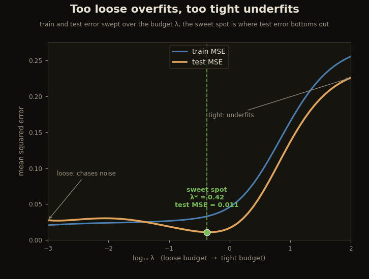
Sweeping gives the empirical trade directly. In the companion run, test MSE reaches its minimum at , where out of forty empirical modes. That number is specific to the sampled Gram matrix, target, noise, and normalization; it is evidence from the sweep, not a generalization theorem derived from effective dimension alone.
The reusable test
A trustworthy spectral companion should pass four checks:
- state the domain and measure;
- construct or verify a positive-definite kernel on that domain;
- keep every eigenvalue nonnegative up to numerical tolerance;
- study partial-norm convergence instead of declaring membership at one cutoff.
With those checks in place, the metaphor becomes exact: the spectrum is a price list, the coefficients are the shopping basket, and the RKHS norm is the bill.
Cite as
Bouhsine, T. (). A Kernel's Price List, in JAX. Records of the !mmortal Data Scientist. https://tahabouhsine.com/blog/what-can-a-weight-be-jax-flax-nnx/
BibTeX
@misc{bouhsine2026whatcanaweightbejaxflaxnnx,
  author       = {Bouhsine, Taha},
  title        = {A Kernel's Price List, in JAX},
  year         = {2026},
  month        = {jun},
  howpublished = {\url{https://tahabouhsine.com/blog/what-can-a-weight-be-jax-flax-nnx/}},
  note         = {Blog post, Records of the !mmortal Data Scientist}
}References
- (1950). Theory of Reproducing Kernels. Transactions of the American Mathematical Society.
- (2004). Scattered Data Approximation. Cambridge University Press.
- (1942). Positive Definite Functions on Spheres. Duke Mathematical Journal.