Metric Learning with Siamese Networks & Triplet Loss

Teach a network a distance, not a label. Instead of predicting a class, a metric-learning model maps inputs to an embedding space where same-class points are close and different-class points are far — perfect for verification, retrieval, clustering, and open-set recognition.

Prerequisites

This is a research-grade guide. It builds directly on contrastive learning — read that first if the idea of "pull positives together, push negatives apart" is new. The embedding backbone is a plain MLP here, but the same recipe drops onto the simple CNN for images.

What you'll learn

• Why metric learning optimizes a distance between embeddings instead of a classification logit
• The triplet loss and the role of the margin, derived and implemented in ~10 lines of JAX
• In-batch hard mining — how to build informative triplets on the fly instead of wasting compute on easy ones
• How L2-normalized embeddings put every point on the unit hypersphere so the margin has a consistent scale
• How supervised metric learning differs from self-supervised SimCLR (labels vs augmentation views)

Example Code

See the full implementation: examples/advanced/metric_learning.py

Why Metric Learning?

A classifier answers "which of these $N$ fixed classes is this?" But many problems don't fit that mold:

• Verification: are these two signatures / faces / fingerprints the same identity? (You may never have seen that identity at training time.)
• Retrieval: given a query, rank a gallery by similarity.
• Few-shot / open-set: new classes appear after training, so a fixed softmax head is useless.

Metric learning sidesteps the fixed label set. It trains an embedding function $f_\theta: x \mapsto z \in \mathbb{R}^d$ so that a simple geometric distance encodes semantic similarity:

$$d(x_a, x_b) = \lVert f_\theta(x_a) - f_\theta(x_b) \rVert_2^2 \quad \text{is small} \iff x_a, x_b \text{ are the same class.}$$

At inference you compare embeddings with a distance — no retraining needed when a new class shows up.

A Siamese network is just weight sharing

The classic picture is two (or three) identical towers with shared weights, one per input. In NNX that sharing is automatic: you define one module and apply it to every input. There is no second copy to keep in sync.

The Triplet Loss

A triplet is $(a, p, n)$: an anchor $a$, a positive $p$ of the same class, and a negative $n$ of a different class. We want the anchor closer to the positive than to the negative, by at least a margin $m$:

$$d(a, p) + m \le d(a, n).$$

Turning that constraint into a hinge loss gives the triplet loss:

$$\mathcal{L}(a, p, n) = \max\!\big(0,\; d(a, p) - d(a, n) + m \big).$$

• If the constraint is already satisfied ($d(a,n) - d(a,p) \ge m$), the loss is exactly $0$ and produces no gradient — the triplet is "easy".
• The margin $m$ sets how much farther the negative must be than the positive. Too small and embeddings collapse; too large and training never reaches zero loss.

Because we L2-normalize embeddings onto the unit sphere, squared distances live in $[0, 4]$, so a margin around $0.2$ is a sensible scale.

The Embedding Network

One shared network, applied to every input, with an L2 normalization on the output:

from shared.models import MLP  # (B, in) -> (B, out)

class EmbeddingNet(nnx.Module):
    """Shared-weight embedding network: input vector -> L2-normalized embedding."""

    def __init__(self, in_features: int, hidden: int, embed_dim: int,
                 *, rngs: nnx.Rngs, depth: int = 2):
        self.backbone = MLP(in_features, hidden, embed_dim, n_layers=depth,
                            rngs=rngs, activation="relu")

    def embed(self, x):
        z = self.backbone(x)
        return z / (jnp.linalg.norm(z, axis=-1, keepdims=True) + 1e-8)

    def __call__(self, x, train: bool = False):
        return self.embed(x)

Normalizing to unit norm is what makes the margin meaningful: without it the network can trivially shrink or inflate all distances and game the loss. Swap MLP for a small CNN and the exact same training code works on images.

In-Batch Hard Mining

Random triplets are mostly easy — the negative is already far, the loss is $0$, and you learn nothing. The fix is mining: build hard triplets from the examples already in the batch. This example uses batch-hard mining (Hermans et al. 2017): for every anchor, pick the farthest positive and the closest negative in the batch.

First, a pairwise squared-distance matrix:

def pairwise_sq_dist(z):
    """Squared Euclidean distance matrix D[i, j] = ||z_i - z_j||^2, shape (B, B)."""
    sq = jnp.sum(z * z, axis=1)
    d = sq[:, None] + sq[None, :] - 2.0 * (z @ z.T)
    return jnp.maximum(d, 0.0)   # clip tiny negatives from round-off

Then mine the hardest positive/negative per anchor using label masks:

def batch_hard_triplet_loss(z, labels, margin: float = 0.2):
    B = z.shape[0]
    D = pairwise_sq_dist(z)

    same = labels[:, None] == labels[None, :]
    eye = jnp.eye(B, dtype=bool)
    pos_mask = same & ~eye          # same class, excluding the anchor itself
    neg_mask = ~same                # different class

    # Hardest positive: largest distance among same-class examples.
    hardest_pos = jnp.max(jnp.where(pos_mask, D, -jnp.inf), axis=1)
    # Hardest negative: smallest distance among different-class examples.
    hardest_neg = jnp.min(jnp.where(neg_mask, D, jnp.inf), axis=1)

    losses = jax.nn.relu(hardest_pos - hardest_neg + margin)
    frac_active = jnp.mean((losses > 0).astype(jnp.float32))
    return jnp.mean(losses), frac_active

The frac_active telemetry — the fraction of anchors with nonzero loss — is worth watching: if it collapses to $0$ too early, the batch has no hard examples left and learning stalls.

Semi-hard vs batch-hard

Batch-hard always takes the closest negative. Semi-hard (the original FaceNet strategy) instead picks a negative that is farther than the positive but still inside the margin: $d(a,p) < d(a,n) < d(a,p)+m$. It avoids a handful of pathological hardest negatives and can be more stable early in training. You can implement it by masking D to that band before the min.

Balanced "PK" batches make mining possible

Mining needs every anchor to have both positives and negatives in the batch. Random shuffling doesn't guarantee that, so sample P classes × K examples each:

def make_pk_batch(X, Y, class_to_idx, P: int, K: int, rng):
    """Sample a balanced batch: P classes, K examples each (batch = P*K)."""
    classes = rng.choice(list(class_to_idx.keys()), size=P, replace=False)
    idxs = []
    for c in classes:
        pool = class_to_idx[int(c)]
        pick = rng.choice(pool, size=K, replace=len(pool) < K)
        idxs.extend(pick.tolist())
    idxs = np.array(idxs)
    return {'x': jnp.asarray(X[idxs]), 'y': jnp.asarray(Y[idxs])}

The Training Step

Standard NNX: differentiate the loss, update in place. The embeddings and mining are computed inside loss_fn so gradients flow through the whole batch of triplets.

@nnx.jit
def train_step(model, optimizer, batch, margin: float = 0.2):
    """One gradient step of triplet-loss metric learning."""
    def loss_fn(model):
        z = model.embed(batch['x'])                       # (B, embed_dim), unit norm
        loss, frac_active = batch_hard_triplet_loss(z, batch['y'], margin)
        return loss, frac_active

    (loss, frac_active), grads = nnx.value_and_grad(loss_fn, has_aux=True)(model)
    optimizer.update(model, grads)
    return loss, frac_active

Measuring Progress: Verification Accuracy

Triplet loss alone is a noisy progress signal — it depends on which hard triplets happen to land in a batch. A cleaner verification metric asks a ranking question directly: for each anchor, is its mean same-class distance smaller than its mean different-class distance?

def verification_accuracy(z, labels):
    B = z.shape[0]
    D = pairwise_sq_dist(z)
    same = labels[:, None] == labels[None, :]
    eye = jnp.eye(B, dtype=bool)
    pos_mask = (same & ~eye).astype(jnp.float32)
    neg_mask = (~same).astype(jnp.float32)

    mean_pos = (D * pos_mask).sum(1) / jnp.maximum(pos_mask.sum(1), 1.0)
    mean_neg = (D * neg_mask).sum(1) / jnp.maximum(neg_mask.sum(1), 1.0)

    acc = jnp.mean((mean_pos < mean_neg).astype(jnp.float32))
    return acc, mean_pos.mean(), mean_neg.mean()

This starts near $0.5$ (random) and climbs toward $1.0$ as the classes separate — a much more stable curve to watch than the raw loss.

Metric Learning vs SimCLR

Metric learning and SimCLR contrastive learning share the "pull together / push apart" intuition, but they differ in where the supervision comes from:

	Metric learning (this page)	SimCLR
Supervision	Labels define positives/negatives	Augmentations define positives
Positive pair	Two examples of the same class	Two augmented views of the same image
Negatives	Different-class examples	All other images in the batch
Loss	Triplet / margin loss	NT-Xent (softmax over similarities)
Needs labels?	Yes	No (self-supervised)

In short: SimCLR invents positives with augmentation because it has no labels; metric learning has labels and uses them to define what "same" means.

Results / What to Expect

By default the script runs fully offline on synthetic class-structured vectors (10 overlapping Gaussian blobs), so it trains in seconds on CPU. Set SYNTHETIC=0 to run on real MNIST (flattened) instead.

python examples/advanced/metric_learning.py

Metric learning (Siamese + triplet loss) on synthetic class-structured vectors
  data: X=(800, 48) classes=10 | in_features=48
  epochs=8 batch=64 (P=8 classes x K=8) embed_dim=32 margin=0.2
  model: EmbeddingNet with 26912 parameters

  epoch  1/8 | step   12 | triplet 0.6823 | active 1.00 | ver_acc 0.885 | d+ 0.204 d- 0.247
  epoch  2/8 | step   24 | triplet 0.3083 | active 1.00 | ver_acc 0.969 | d+ 0.083 d- 0.106
  epoch  4/8 | step   48 | triplet 0.2314 | active 1.00 | ver_acc 0.979 | d+ 0.038 d- 0.050
  epoch  6/8 | step   72 | triplet 0.2199 | active 1.00 | ver_acc 0.990 | d+ 0.026 d- 0.035
  epoch  8/8 | step   96 | triplet 0.2144 | active 1.00 | ver_acc 0.990 | d+ 0.020 d- 0.027

Done. The embedding pulls same-class inputs together and pushes different-class inputs apart (d+ < d-).

The triplet loss falls (0.68 → 0.21), the mean same-class distance d+ stays below the mean different-class distance d-, and verification accuracy rises toward 0.99. The loss plateaus near the margin because batch-hard mining keeps surfacing the toughest remaining triplets — that residual is expected, not a bug.

The script also saves a 2D PCA projection of the embeddings, comparing random initialization to the trained model:

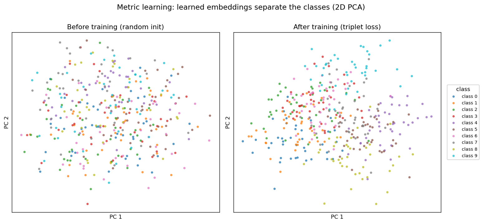
Each point is one input, colored by its true class. At random initialization (left) the classes are thoroughly mixed; after training (right) same-class points cluster together and different classes occupy distinct regions — visual proof that the network learned a metric where distance encodes class identity.

Common Pitfalls

1. Forgetting to normalize embeddings ❌ The network cheats by scaling all distances, and the margin loses meaning. ✅ L2-normalize the output (unit hypersphere) so the margin has a fixed, interpretable scale.

2. Random triplets instead of mining ❌ Most random triplets are already easy → loss $\approx 0$ → no gradient → glacial training. ✅ Mine hard (or semi-hard) triplets within the batch so every step has signal.

3. Unbalanced batches ❌ A shuffled batch may give an anchor zero same-class peers, so mining has no positive. ✅ Sample balanced P classes × K examples batches so positives and negatives always exist.

4. Margin set wrong ❌ Too large → loss never reaches zero and embeddings never tighten; too small → representations collapse to a point. ✅ Start around $m = 0.2$ for unit-norm embeddings and tune while watching frac_active.

5. Judging progress by loss alone ❌ Batch-hard loss is noisy and plateaus near the margin, which looks like "stuck". ✅ Track a verification / retrieval metric (positive pairs closer than negatives) as the real signal.

Next steps

• Contrastive Learning with SimCLR — the self-supervised cousin that invents positives from augmentations instead of labels.
• Advanced Techniques — more research-grade training recipes and the Research hub.
• Simple CNN — swap the MLP backbone for a conv net to do metric learning on images.

Complete Example

Siamese + triplet-loss metric learning:

• examples/advanced/metric_learning.py — shared-weight embedding network, batch-hard triplet loss, balanced PK sampling, and a verification metric. Runs offline on synthetic data by default; SYNTHETIC=0 switches to MNIST.

References

• FaceNet: A Unified Embedding for Face Recognition and Clustering (Schroff et al., CVPR 2015) — introduced the triplet loss with semi-hard mining.
• In Defense of the Triplet Loss: In Defense of the Triplet Loss for Person Re-Identification (Hermans et al., 2017) — the batch-hard mining strategy used here.
• Contrastive loss (Siamese): Dimensionality Reduction by Learning an Invariant Mapping (Hadsell, Chopra & LeCun, CVPR 2006) — the original margin-based pairwise loss.
• Sampling Matters: Sampling Matters in Deep Embedding Learning (Wu et al., ICCV 2017) — why negative mining/sampling drives embedding quality.