Cheap Attention in JAX/Flax NNX
#ml#attention#kernels#linear-attention#performer#jax#flax#nnx#implementation#transformers#random-features
Part 3 of 6Attention Is a Kernel
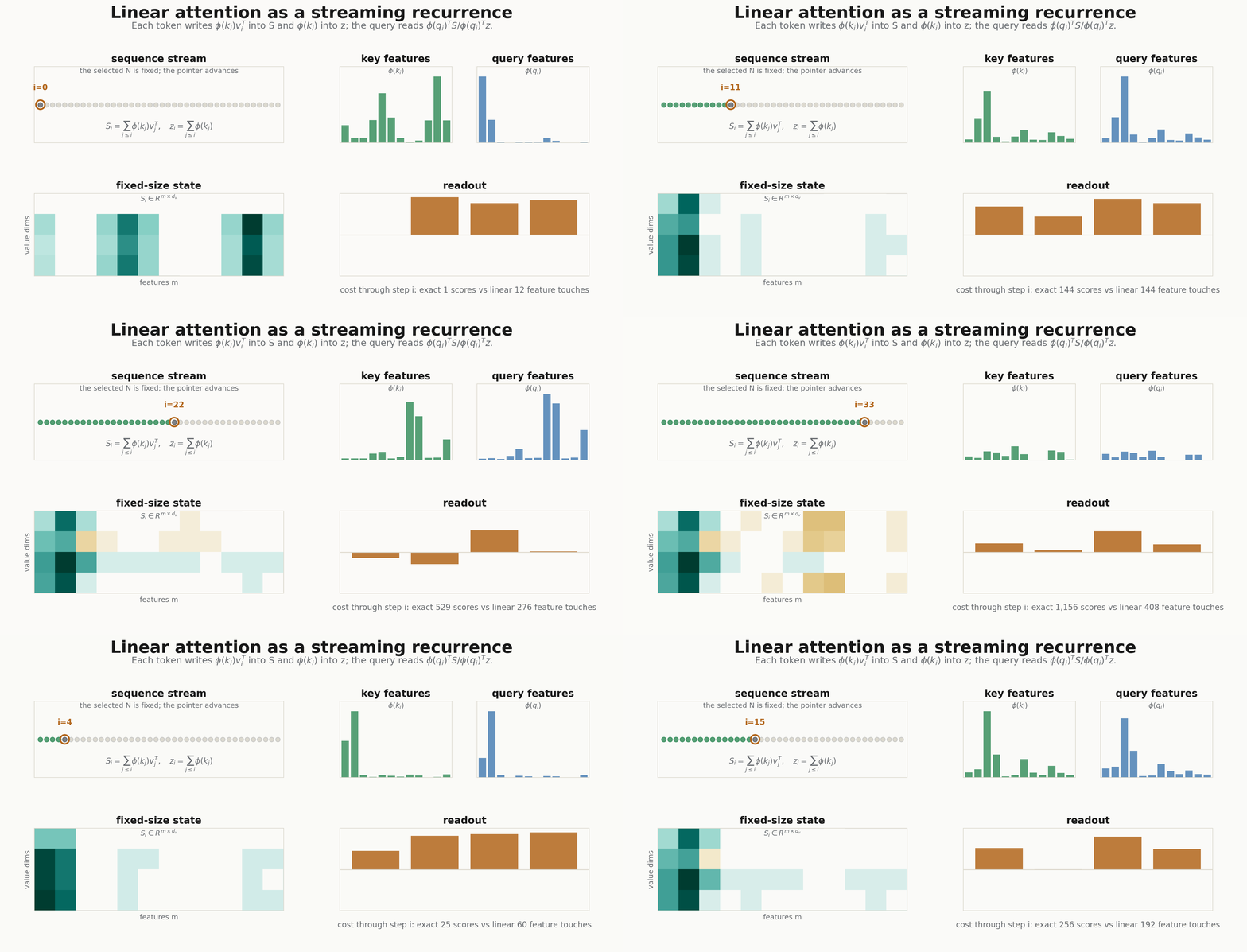
Where does the table actually go? The theory post answers in algebra: pick a finite feature map, then move one pair of parentheses. Here that answer is arrays you can print, a Flax NNX module you can drop into a model, a causal recurrence that decodes one token at a time, and animations that follow the bookkeeping as it stops being an all-pairs ledger and becomes a shared state.
Prefer a notebook? Run the whole thing on Kaggle: the same code, block by block, with the math written out and every figure reproduced from a real run.
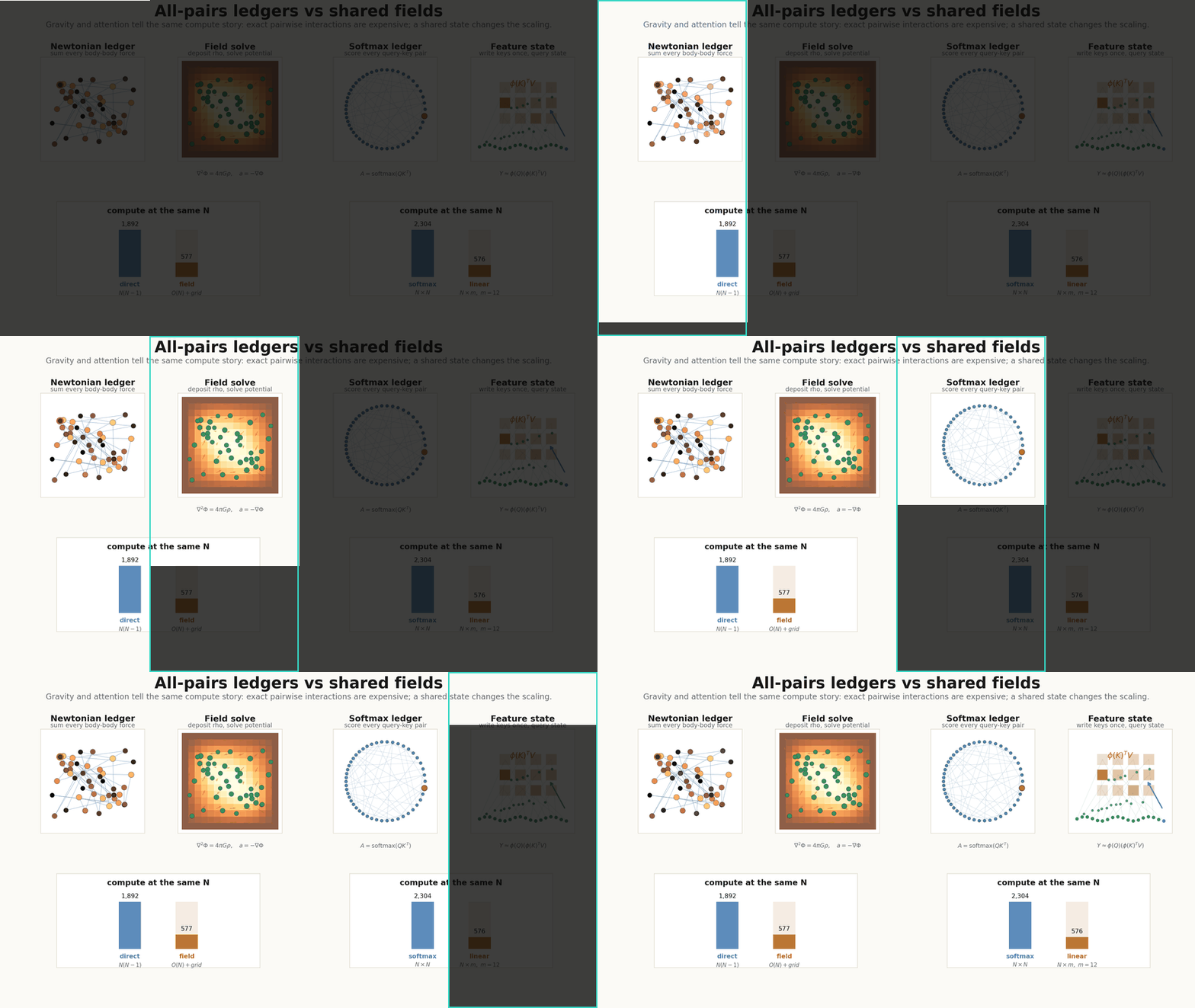
The companion to Cheap Attention: Linear-Time Kernel Approximation should be boring in the best way. No custom CUDA, no special kernel, no hidden magic. Just three JAX operations:
- Project tokens into .
- Replace with a positive random feature dot product .
- Compute before multiplying by .
That third line is the whole implementation story. Exact softmax attention does
so the score table sits in the middle. Linear attention does
so the middle object is no longer token-by-token. It is a feature-space state.
The feature map
Everything hinges on one choice: which stands in for the softmax kernel’s infinite one? The Performer’s answer is positive random features:
The positivity matters because these numbers become attention weights before normalization. A trig feature map can be unbiased and still put negative mass into a row. Positive features keep the denominator meaningful.
In JAX, the feature map is one einsum plus the norm correction:
import jax.numpy as jnp

def positive_features(x, omega):
    """x: [..., d_head], omega: [m, d_head] -> [..., m]."""
    proj = jnp.einsum("...d,md->...m", x, omega)
    norm = 0.5 * jnp.sum(x * x, axis=-1, keepdims=True)
    return jnp.exp(proj - norm) / jnp.sqrt(omega.shape[0])
For a multi-head implementation, each head can own its own random matrix:
def head_features(x, omega):
    """x: [batch, tokens, heads, d_head], omega: [heads, m, d_head]."""
    proj = jnp.einsum("bthd,hmd->bthm", x, omega)
    norm = 0.5 * jnp.sum(x * x, axis=-1, keepdims=True)
    return jnp.exp(proj - norm) / jnp.sqrt(omega.shape[1])
Check it against exact attention
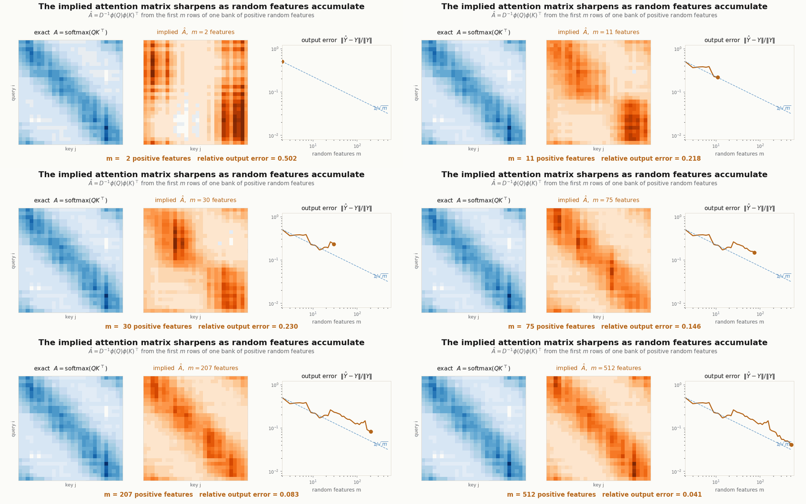
Does the reassociated product actually compute attention, or just something attention-shaped? Both versions are a few lines, so verify instead of trusting: build one set of queries, keys, and values, compute exact softmax attention, then compute the linear version at increasing and watch the error fall.
def exact_attention(q, k, v):
    return jax.nn.softmax(jnp.einsum("id,jd->ij", q, k), axis=-1) @ v


def linear_attention(q, k, v, omega):
    phi_q, phi_k = positive_features(q, omega), positive_features(k, omega)
    kv = jnp.einsum("tm,td->md", phi_k, v)     # the shared state, [m, d]
    z = phi_k.sum(axis=0)                      # the shared normalizer, [m]
    return jnp.einsum("tm,md->td", phi_q, kv) / (phi_q @ z)[:, None]


N, d = 64, 16
kq, kk, kv, ko = jax.random.split(jax.random.key(0), 4)
q = jax.random.normal(kq, (N, d)) / jnp.sqrt(d)   # unit-ish norms, like trained q/k
k = jax.random.normal(kk, (N, d)) / jnp.sqrt(d)
v = jax.random.normal(kv, (N, d))

y = exact_attention(q, k, v)
for m in (16, 64, 256, 1024):
    errs = []
    for s in range(20):   # 20 independent feature draws
        omega = jax.random.normal(jax.random.fold_in(jax.random.fold_in(ko, m), s), (m, d))
        y_hat = linear_attention(q, k, v, omega)
        errs.append(jnp.linalg.norm(y_hat - y) / jnp.linalg.norm(y))
    errs = jnp.stack(errs)
    print(f"m = {m:4d}   relative error {errs.mean():.3f}   (worst draw {errs.max():.3f})")
A real run of this block prints:
m =   16   relative error 0.480   (worst draw 0.611)
m =   64   relative error 0.295   (worst draw 0.480)
m =  256   relative error 0.183   (worst draw 0.259)
m = 1024   relative error 0.099   (worst draw 0.134)
Each 4x in features roughly halves the error: the behavior of a Monte Carlo estimate, visible in the digits. The measured rate uses unit-norm queries and keys. Because the positive-feature estimator’s variance grows like , larger norms require more features or variance-reduction constructions such as orthogonal features.
The NNX module
So where does the verified feature map live in a real model? In an ordinary Flax NNX module: a plain Python object that subclasses nnx.Module, with submodules like nnx.Linear assigned as attributes in __init__. Randomness is handled with nnx.Rngs, which is passed at initialization to create parameters.
Here is a compact non-causal linear-attention layer. It is the direct translation of the algebra above.
from flax import nnx
import jax
import jax.numpy as jnp

class LinearAttention(nnx.Module):
    def __init__(
        self,
        d_model: int,
        n_heads: int,
        n_features: int,
        *,
        rngs: nnx.Rngs,
    ):
        assert d_model % n_heads == 0
        self.d_model = d_model
        self.n_heads = n_heads
        self.d_head = d_model // n_heads
        self.n_features = n_features

        self.q = nnx.Linear(d_model, d_model, rngs=rngs)
        self.k = nnx.Linear(d_model, d_model, rngs=rngs)
        self.v = nnx.Linear(d_model, d_model, rngs=rngs)
        self.o = nnx.Linear(d_model, d_model, rngs=rngs)

        omega = jax.random.normal(
            rngs.params(),
            (n_heads, n_features, self.d_head),
        )
        self.omega = nnx.Param(omega)

    def split_heads(self, x):
        b, t, _ = x.shape
        return x.reshape(b, t, self.n_heads, self.d_head)

    def positive_features(self, x):
        proj = jnp.einsum("bthd,hmd->bthm", x, self.omega[...])
        norm = 0.5 * jnp.sum(x * x, axis=-1, keepdims=True)
        return jnp.exp(proj - norm) / jnp.sqrt(self.n_features)

    def __call__(self, x, eps=1e-6):
        q = self.split_heads(self.q(x))
        k = self.split_heads(self.k(x))
        v = self.split_heads(self.v(x))

        phi_q = self.positive_features(q)  # [b, t, h, m]
        phi_k = self.positive_features(k)  # [b, t, h, m]

        # Shared feature-state. This is the line where N x N disappears.
        kv = jnp.einsum("bthm,bthd->bhmd", phi_k, v)
        z = jnp.sum(phi_k, axis=1)

        num = jnp.einsum("bthm,bhmd->bthd", phi_q, kv)
        den = jnp.einsum("bthm,bhm->bth", phi_q, z)[..., None]
        y = num / (den + eps)

        return self.o(y.reshape(x.shape))
The important shape is kv: [batch, heads, m, d_head]. It does not contain a token-token axis. Exact attention’s middle object is [batch, heads, tokens, tokens]; linear attention’s middle object is [batch, heads, features, head_dim].
Causal decoding
For autoregressive decoding, the recurrence is even more explicit. At step :
For a whole training sequence, cumsum is the easiest way to write it:
def causal_linear_attention(phi_q, phi_k, v, eps=1e-6):
    """phi_*: [batch, tokens, heads, m], v: [batch, tokens, heads, d]."""
    kv = jnp.einsum("bthm,bthd->bthmd", phi_k, v)
    s = jnp.cumsum(kv, axis=1)
    z = jnp.cumsum(phi_k, axis=1)

    num = jnp.einsum("bthm,bthmd->bthd", phi_q, s)
    den = jnp.einsum("bthm,bthm->bth", phi_q, z)[..., None]
    return num / (den + eps)
For one-token-at-a-time generation, you do not need the full prefix arrays:
def decode_step(phi_q_i, phi_k_i, v_i, state, eps=1e-6):
    """One recurrent decoding step.

    phi_q_i, phi_k_i: [batch, heads, m]
    v_i:              [batch, heads, d]
    state.s:          [batch, heads, m, d]
    state.z:          [batch, heads, m]
    """
    s = state.s + jnp.einsum("bhm,bhd->bhmd", phi_k_i, v_i)
    z = state.z + phi_k_i
    num = jnp.einsum("bhm,bhmd->bhd", phi_q_i, s)
    den = jnp.einsum("bhm,bhm->bh", phi_q_i, z)[..., None]
    return num / (den + eps), state.replace(s=s, z=z)
That is the recurrent-network view: the cache is no longer all past keys and values. It is a fixed feature state.
Train it on a routing task
Approximation error is one question; the sharper one is whether gradients can learn through the approximation. A tiny task settles it. Each training sequence is 48 random vectors, one of which is marked by a flag channel, and the target is for every position to output the marked token’s content. Solving it means routing one token’s content to all the others, which is precisely the job attention exists to do.
The layer is an ordinary nnx.Module, so it drops into the standard NNX loop (with current NNX, nnx.Optimizer takes wrt=nnx.Param, and update receives both the model and the gradients):
import optax

d_model, N = 32, 48

def routing_batch(key, batch=64):
    kx, km = jax.random.split(key)
    x = jax.random.normal(kx, (batch, N, d_model))
    marked = jax.random.randint(km, (batch,), 0, N)
    x = x.at[jnp.arange(batch), marked, 0].set(4.0)          # the flag channel
    target = jnp.repeat(x[jnp.arange(batch), marked][:, None, :], N, axis=1)
    return x, target

model = LinearAttention(d_model=d_model, n_heads=2, n_features=64, rngs=nnx.Rngs(0))
optimizer = nnx.Optimizer(model, optax.adamw(1e-3), wrt=nnx.Param)

@nnx.jit
def train_step(model, optimizer, batch):
    x, target = batch

    def loss_fn(model):
        return jnp.mean((model(x) - target) ** 2)

    loss, grads = nnx.value_and_grad(loss_fn)(model)
    optimizer.update(model, grads)
    return loss

key = jax.random.key(42)
for step in range(1001):
    key, sub = jax.random.split(key)
    loss = train_step(model, optimizer, routing_batch(sub))
    if step % 250 == 0:
        print(f"step {step:4d}   loss {loss:.3f}")
A real run of this loop prints:
step    0   loss 1.790
step  250   loss 0.989
step  500   loss 0.519
step  750   loss 0.059
step 1000   loss 0.003
The layer learns to find the flag and broadcast the marked content, and nothing about the loop knows it is training an approximation: the gradient just flows through , through the shared state, through the ratio. The implementation choice to watch is not jit; it is the tensor you permit yourself to create. If your forward pass forms scores = q @ k.T, you are back in the ledger world. If it forms kv = phi_k.T @ v, you have crossed into the shared-state world.
How the animations are computed
All three GIFs in this post are generated with Python, JAX, and matplotlib. The gravity animation computes:
- direct softened Newtonian -body accelerations with JAX,
- a particle-mesh Poisson solve with
jnp.linalg.solve, - exact attention scores,
- and a finite-feature attention state.
The pipeline animation follows the causal linear-attention recurrence token by token, and the error animation recomputes the exact and implied attention matrices at every feature count . They are deliberately small: the point is not a benchmark, but a visual audit of the shapes. If the GIF cannot show where the object disappeared, the implementation is probably not explaining itself.
Boundary of the result
This is a teaching implementation, not a production kernel. A production version would care about:
- orthogonal random features instead of plain Gaussian draws,
- numerical stabilization around the exponential features,
- efficient scan kernels for causal training,
- mixed precision policy,
- and whether the target workload actually tolerates the approximation.
Those choices matter. But they are second-order to the core idea. Linear attention is not “attention but faster” by accident. It is attention after you choose a finite feature map and refuse to materialize the pairwise ledger.
References: Flax NNX Module API and randomness guide; Performer / FAVOR+ from Choromanski et al. (2021); linear-transformer recurrence from Katharopoulos et al. (2020).
Cite as
Bouhsine, T. (). Cheap Attention in JAX/Flax NNX. Records of the !mmortal Data Scientist. https://tahabouhsine.com/blog/linear-attention-jax-flax-nnx/
BibTeX
@misc{bouhsine2026linearattentionjaxflaxnnx,
  author       = {Bouhsine, Taha},
  title        = {Cheap Attention in JAX/Flax NNX},
  year         = {2026},
  month        = {may},
  howpublished = {\url{https://tahabouhsine.com/blog/linear-attention-jax-flax-nnx/}},
  note         = {Blog post, Records of the !mmortal Data Scientist}
}References
- (2020). Transformers are RNNs: Fast Autoregressive Transformers with Linear Attention. ICML 2020.arXiv:2006.16236
- (2021). Rethinking Attention with Performers. ICLR 2021.arXiv:2009.14794