Running the Survival Trial, in JAX/Flax NNX

The explainer put a deep Yat-kernel survival model on trial across five real datasets: viable, in the pack on the mid-sized problems, behind on the small and the near-separable ones, and carrying a theory the baselines do not have. This is the machinery underneath it: the Yat DeepSurv trunk in Flax NNX, the Cox partial-likelihood loss, the learning-rate-fair training loop that keeps the neural comparison fair, the concordance / integrated-Brier / time-dependent-AUC evaluation, and the classical baselines wired through scikit-survival. Every figure is a real number from scripts/deepsurv_trial.py; this is a research illustration, not a clinical tool.

The trunk is the only thing that changes#

A DeepSurv is a loss with a hole in it: any network that maps a patient to one scalar log-risk can be dropped into the Cox partial likelihood and trained. The standard recipe fills the hole with a ReLU MLP; the white-box model fills it with a bank of Yat kernels, and nothing else about the pipeline moves. So both trunks are two short modules with the same signature.

import jax, jax.numpy as jnp
from flax import nnx

class YatLayer(nnx.Module):
    """K prototype kernels: phi_u(x) = (w_u . x + b)^2 / (||x - w_u||^2 + eps)."""
    def __init__(self, d_in, k, *, Winit):
        self.W = nnx.Param(jnp.asarray(Winit))                 # [K, d] prototypes, in input space
        self.log_b = nnx.Param(jnp.full((), jnp.log(jnp.expm1(1.0))))
        self.log_eps = nnx.Param(jnp.full((), jnp.log(jnp.expm1(1.0))))

    def __call__(self, x):
        b = jax.nn.softplus(self.log_b.value); eps = jax.nn.softplus(self.log_eps.value)
        dot = x @ self.W.value.T
        d2 = jnp.sum(x**2, -1, keepdims=True) + jnp.sum(self.W.value**2, -1) - 2 * dot
        return (dot + b) ** 2 / (d2 + eps)                     # [n, K] bounded kernel activations

class YatSurv(nnx.Module):
    """Yat DeepSurv: prototype-kernel trunk -> one scalar log-risk."""
    def __init__(self, d_in, k, *, rngs, Winit):
        self.yat = YatLayer(d_in, k, Winit=Winit)
        self.read = nnx.Linear(k, 1, use_bias=False, rngs=rngs)

    def __call__(self, x):
        return self.read(self.yat(x))[:, 0]                    # h(x) = sum_u a_u phi_u(x)

The Winit argument is where the legibility is decided. The prototypes are seeded on real patients (k-means centroids of the training cohort), so from the first step every hidden unit is a point in patient space rather than an opaque direction. The standard DeepSurv is the same file with a two-layer ReLU MLP in place of YatLayer, and its Winit argument does not exist, which is exactly the difference the trial is about.

The loss decides who ranks above whom#

The loss does not care which trunk produced the log-risks. At each observed death, the patient who died should have outscored everyone still at risk at that moment; sort by descending time and each risk set becomes a running prefix, so the log of the risk-set sum is a cumulative logsumexp from the top.

def cox_ph_loss(logrisk, times, events):
    """Negative Cox partial log-likelihood (Breslow ties)."""
    order = jnp.argsort(-times)                                  # descending time
    h = logrisk[order]; ev = events[order]
    m = jnp.max(h)                                               # stabilize the logsumexp
    log_cum = m + jnp.log(jnp.cumsum(jnp.exp(h - m)) + 1e-12)    # log sum over each risk set
    return -jnp.sum((h - log_cum) * ev) / (jnp.sum(ev) + 1e-8)

Only observed events contribute a term, but censored patients are not thrown away: they sit inside the risk-set sums of every death before their censoring time. That is how the partial likelihood uses a patient you only watched for a while without inventing a death date.

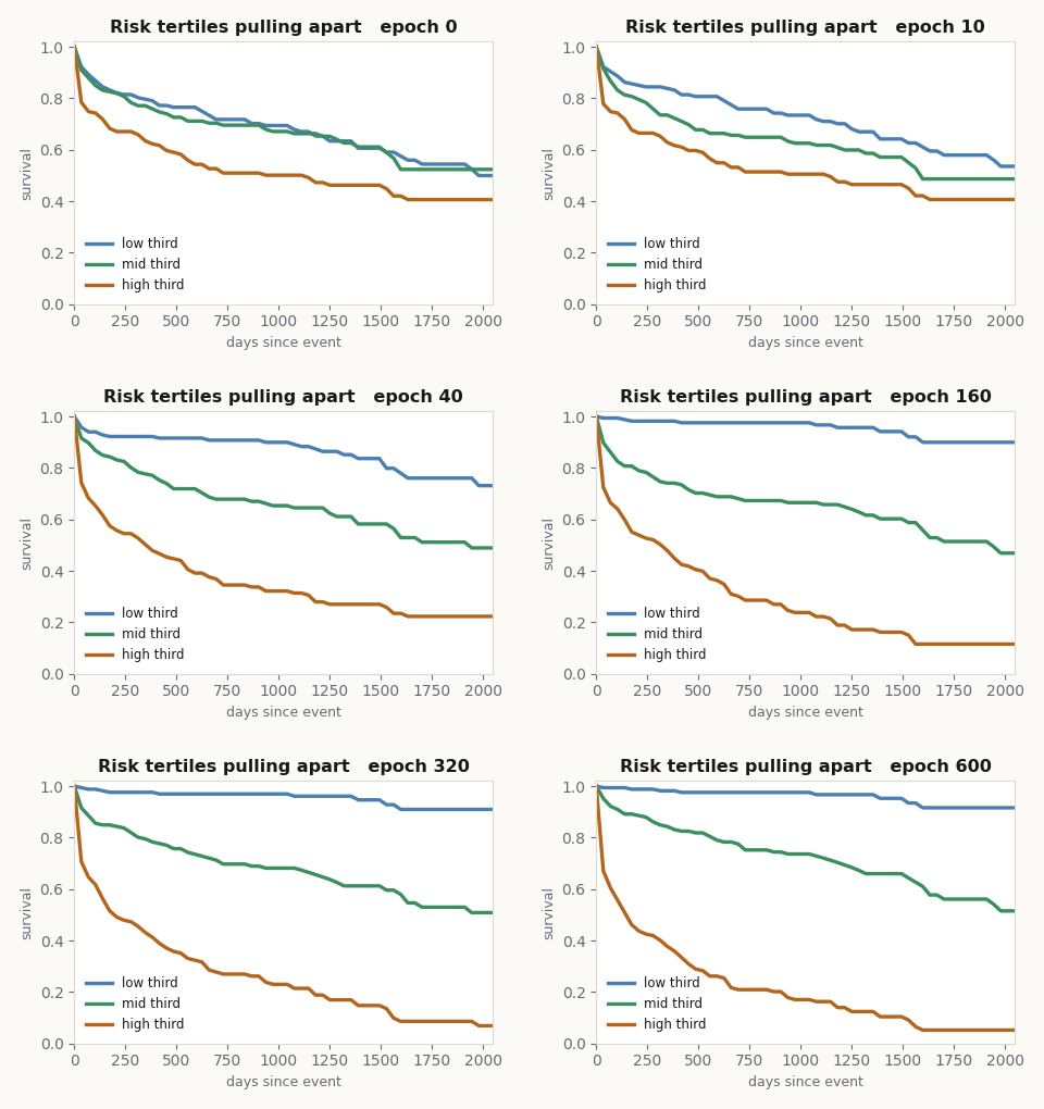
Here is that loss doing its work. On the WHAS500 cohort, training the real Yat DeepSurv from scratch, the three risk tertiles start on top of each other and pull apart as the log-risks find their order. Nothing in this animation is staged: each frame is a real Kaplan-Meier estimate on the tertiles the model’s current risk scores define.

LR-fairness is the whole ballgame in a neural comparison#

Why not train both nets at one learning rate and be done? Because a shared rate measures the optimizer, not the model. A convergence probe found the Yat trunk and the ReLU MLP prefer different rates, so the comparison lets each net sweep its own grid, pick the rate that maximizes an inner-validation concordance, and stop at that candidate’s best epoch, all without ever touching the test set.

def select_and_fit_net(build_fn, sp, lr_grid=(3e-3, 1e-2, 3e-2)):
    """Sweep the learning rate; keep the model with the best inner-validation C-index,
    each candidate early-stopped at its own best epoch. The test set is untouched."""
    best = None
    for lr in lr_grid:
        model = build_fn()                                      # a fresh trunk of this kind
        model, val_c, best_ep = train_net(model, sp, lr=lr)     # best-epoch on inner val
        if best is None or val_c > best["val_c"]:
            best = dict(model=model, lr=lr, val_c=val_c, best_ep=best_ep)
    return best                                                 # reported at its OWN best lr

The inner training loop is plain AdamW on the Cox loss, snapshotting whenever the validation concordance improves and restoring that snapshot at the end, so neither net is ever judged on an over-trained endpoint.

import optax

@nnx.jit
def train_step(model, opt, xb, tb, eb):
    def loss_fn(m): return cox_ph_loss(m(xb), tb, eb)
    loss, grads = nnx.value_and_grad(loss_fn)(model)
    opt.update(model, grads)
    return loss

def train_net(model, sp, *, lr, epochs=800, val_every=25):
    opt = nnx.Optimizer(model, optax.adamw(lr, weight_decay=1e-4), wrt=nnx.Param)
    Xj, tj, ej = map(jnp.asarray, (sp["Xtrn"], sp["ttrn"], sp["etrn"]))
    best_c, best_snap = -jnp.inf, None
    for ep in range(1, epochs + 1):
        train_step(model, opt, Xj, tj, ej)
        if ep % val_every == 0:
            c = c_index(model, sp["Xval"], sp["tval"], sp["eval"])   # inner-val concordance
            if c > best_c: best_c, best_snap = c, snapshot(model)
    restore(model, best_snap)
    return model, float(best_c), ep

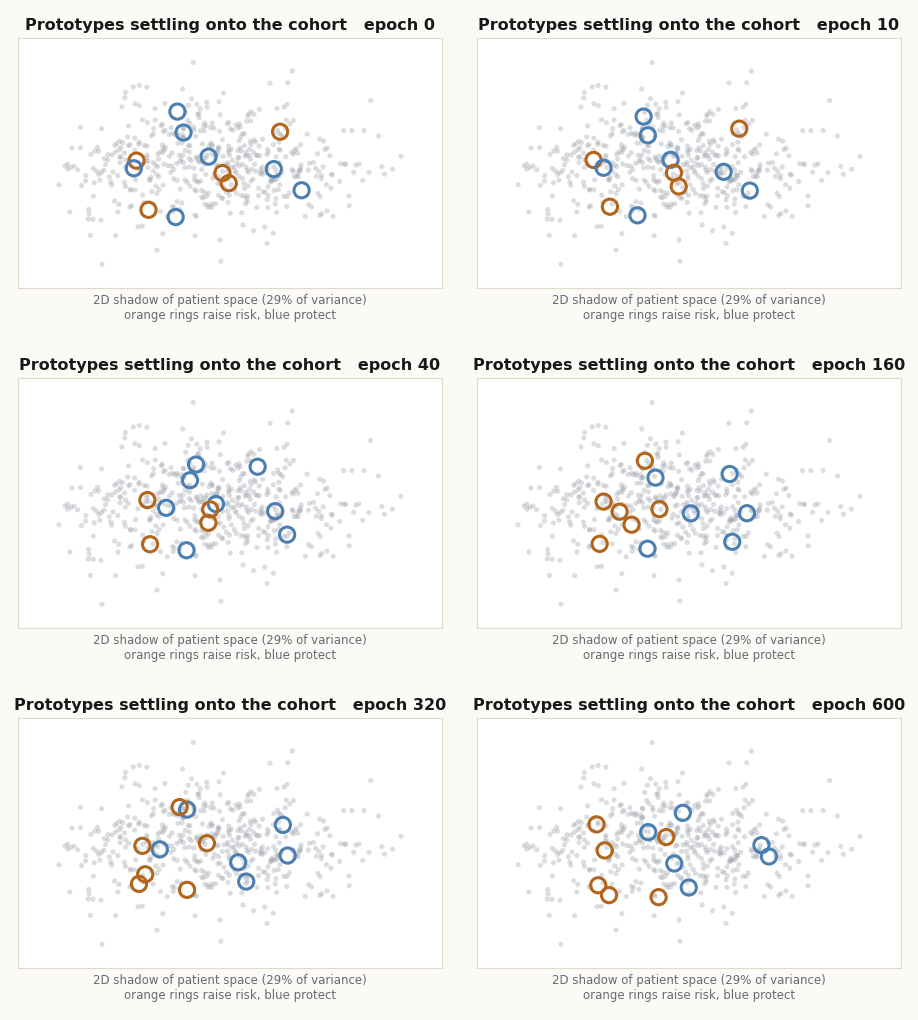
Because the prototypes start on real patients, you can watch the trunk do something the MLP cannot: the prototype cloud migrates across the patient space as the model fits, each ring a synthetic patient sliding toward where the risk signal wants it. The rings are the real model.yat.W at each captured epoch, projected onto a fixed 2D shadow of the cohort, so the motion is the fit and nothing else.

The metric quartet, and why one number is not enough#

A concordance index answers “did it rank right,” and nothing else, so the trial computes four things per model. Harrell’s C measures ranking; the time-dependent AUC measures ranking at fixed horizons; the integrated Brier score (Graf et al., 1999) measures whether the predicted probabilities are any good; and the held-out Cox likelihood measures the loss itself. All four come straight out of scikit-survival once you have a risk score and a survival function.

from sksurv.metrics import (concordance_index_censored,
                            cumulative_dynamic_auc, integrated_brier_score)

def c_index(model, X, tt, ee):
    r = np.asarray(model(jnp.asarray(X)))                      # log-risk, higher = higher risk
    return concordance_index_censored(ee.astype(bool), tt, r)[0]

# survival curves from a Breslow baseline hazard let us score AUC and Brier too
S_te = breslow_survival(risk_tr, risk_te, sp)                  # [n_test, horizons]
_, mean_auc = cumulative_dynamic_auc(y_tr, y_te, risk_te, horizons)
ibs = integrated_brier_score(y_tr, y_te, S_te, horizons)

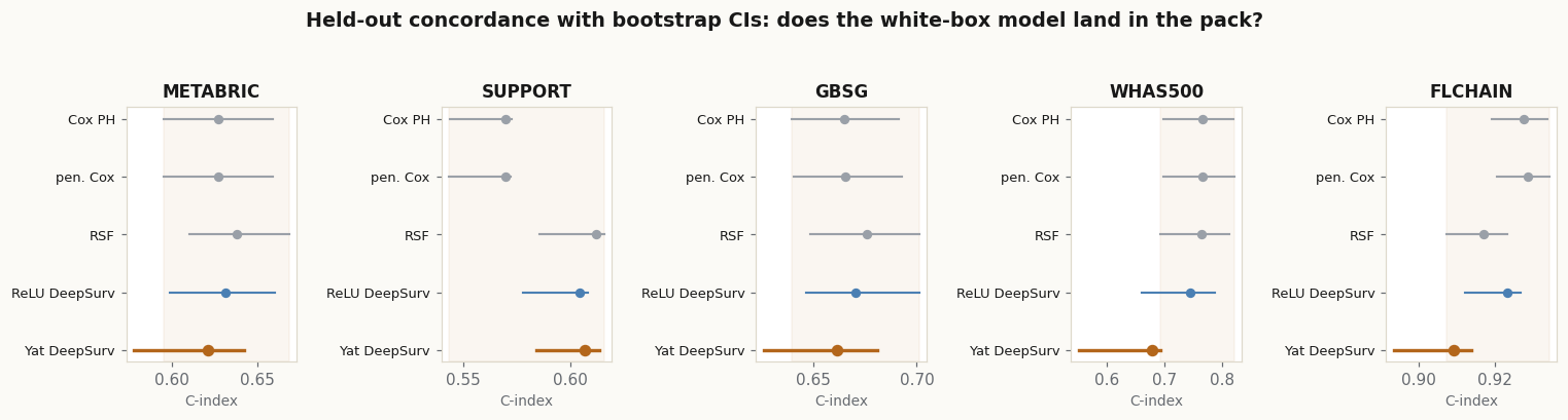
Running that across five datasets, six seeds, with a 300-resample bootstrap on the test concordance, is the whole viability result in one figure. Each point is a model’s mean C-index; the whisker is its bootstrap interval; the shaded band is the classical baselines’ envelope, so “in the pack” is literally the shaded region.

The baselines are three lines each#

The classical models exist so the comparison has an anchor with no learning rate to argue about. scikit-survival gives all three a .predict that returns a risk score with the same orientation as the neural log-risk, so the same evaluation code scores every model.

from sksurv.linear_model import CoxPHSurvivalAnalysis, CoxnetSurvivalAnalysis
from sksurv.ensemble import RandomSurvivalForest

def fit_classical(kind, sp, seed):
    y_tr = Surv.from_arrays(event=sp["etr"].astype(bool), time=sp["ttr"])
    est = {"coxph":  CoxPHSurvivalAnalysis(alpha=1e-2),                    # tiny ridge for stability
           "coxnet": CoxnetSurvivalAnalysis(l1_ratio=0.5, max_iter=100000),
           "rsf":    RandomSurvivalForest(n_estimators=200, min_samples_leaf=15,
                                          max_features="sqrt", random_state=seed)}[kind]
    est.fit(sp["Xtr"], y_tr)
    return est.predict(sp["Xtr"]), est.predict(sp["Xte"])                  # risk scores, higher = riskier

One subtlety lives in this function: the Random Survival Forest’s risk score is not a Cox log-hazard, so its partial likelihood is not comparable to the Cox-family models and the trial drops it rather than print a meaningless number. The concordance, AUC and Brier are all comparable, so those it keeps.

Stability, calibration, strangers, and plausibility, each a short slice#

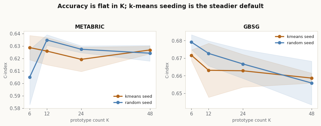
The rest of the trial is the inheritance the explainer walks through, and each piece is a small operation on the arrays you already have. The prototype-count ablation just rebuilds the trunk with different K and Winit and re-scores; the answer is that accuracy barely moves and k-means seeding is the steadier default.

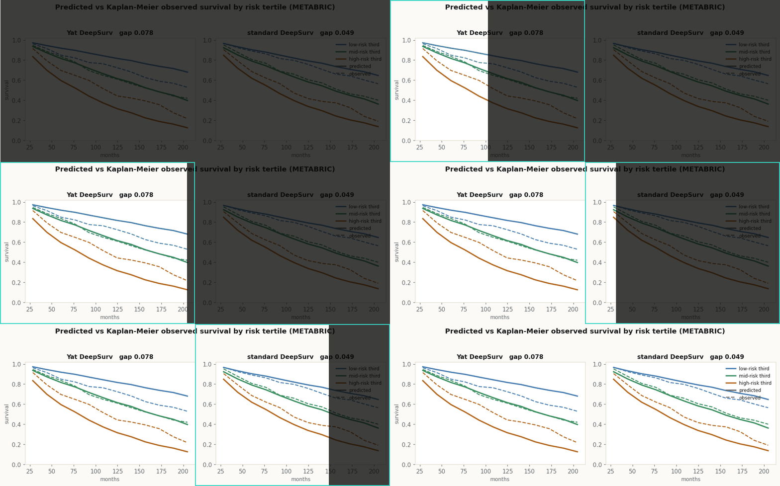
Calibration is the survival curve read back against reality: bin the held-out patients into risk tertiles and compare each tertile’s mean predicted survival to its Kaplan-Meier estimate at a set of horizons. Closer curves are probabilities you can trust.

The out-of-distribution meter is a single max over the kernel activations, and the split is the point: scored across five datasets and three constructions, some bars land above 0.5 (the meter flags a stranger) and some land below (it does not, because the shift is mild or a far-tail point still falls near a prototype).

kmax_in  = phi_test.max(1)                                     # resemblance meter on real patients
kmax_ood = model.yat(jnp.asarray(X_ood)).max(1)               # ... on a constructed outsider
auroc = roc_auc_score(np.r_[np.ones_like(kmax_in), np.zeros_like(kmax_ood)],
                      np.r_[kmax_in, kmax_ood])               # high AUROC = strangers score low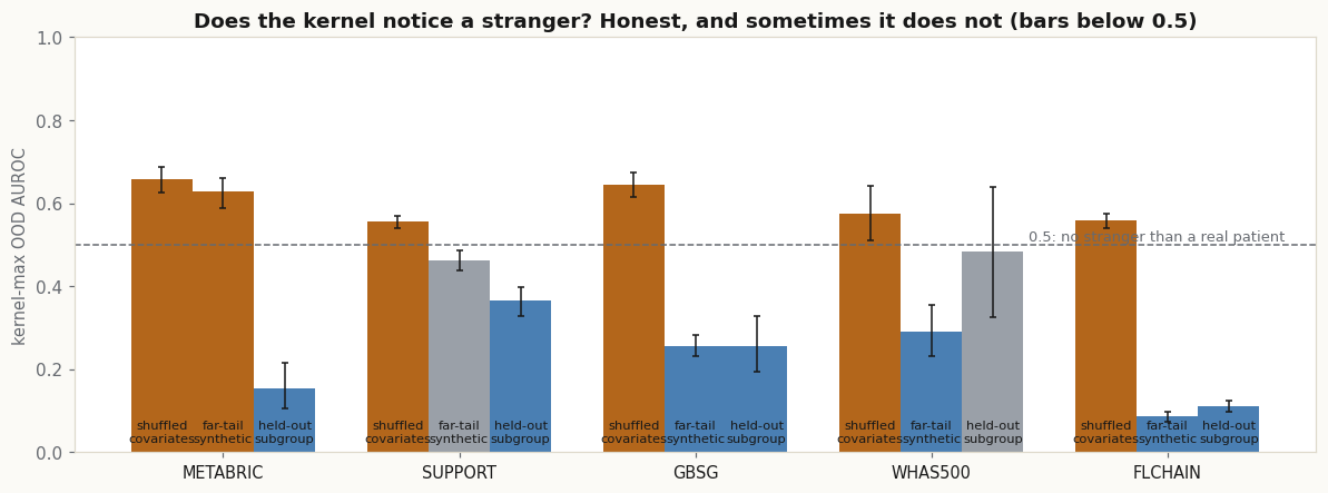

Plausibility is a de-normalization and a range check: multiply each prototype by the training standard deviation, add the mean, and ask whether every covariate lands inside the observed min and max. The excursions concentrate on the binary treatment indicators a continuous prototype cannot represent cleanly, while the gene-expression and age covariates stay in range.

W_clin = model.yat.W.value * sd + mu                          # prototypes back in clinical units
in_range = (model.yat.W.value >= X_tr.min(0)) & (model.yat.W.value <= X_tr.max(0))
frac_plausible = (in_range.all(1)).mean()                     # share of fully in-range prototypes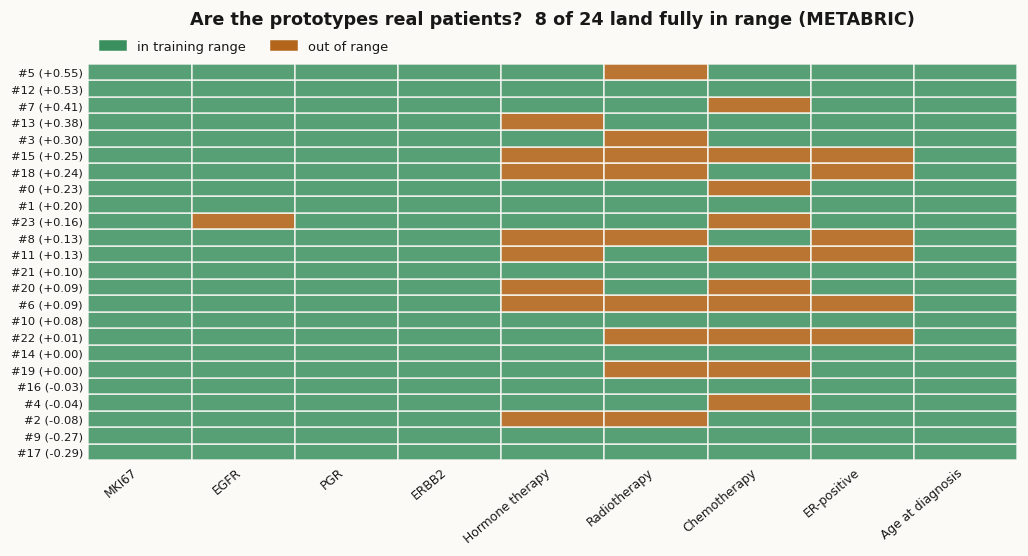

That is the whole trial: one loss, two trunks, three classical baselines, and a handful of array operations that turn a single log-risk into a ranking, a calibration, an abstention, and an audit. The results and the full reading of them live in the explainer.

@misc{bouhsine2026survivalmodelontrialjaxflaxnnx,
  author       = {Bouhsine, Taha},
  title        = {Running the Survival Trial, in JAX/Flax NNX},
  year         = {2026},
  month        = {jul},
  howpublished = {\url{https://tahabouhsine.com/blog/survival-model-on-trial-jax-flax-nnx/}},
  note         = {Blog post, Records of the !mmortal Data Scientist}
}