Constructing the Fashion-MNIST Network, in JAX/Flax NNX

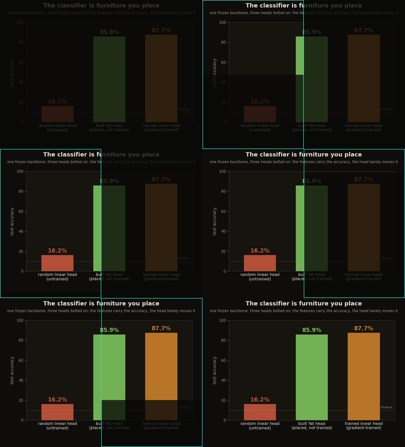
The head in this post is a function, not a module. That is the shortest way to state what the explainer was arguing: split a network into a backbone that builds features and a head that classifies, train only the backbone, and the classifier can be placed by hand rather than fitted. So there are two pieces of code here, a small Flax NNX convolutional network with an ordinary training loop, and fifteen lines of k-means and kernel arithmetic that never see a gradient. Run both on the same frozen features and the gap between them is where the argument lives: 85.9% against 87.7%, measured here.

Prefer a notebook? Run the whole thing on Kaggle: the same code, block by block, with the math written out and every figure reproduced from a real run.

The two stages, as two modules#

Where does the explainer’s split land in code? In two modules. The backbone is the part we train, two conv-and-pool blocks down to a 64-dimensional feature; the head is a plain linear layer for the trained baseline, and later a placed Yat vote for the constructed version.

import jax, jax.numpy as jnp, optax
from flax import nnx

class Backbone(nnx.Module):
    """Two conv-pool blocks to a 64-d feature. This is the only part that gets trained."""
    def __init__(self, rngs):
        self.c1 = nnx.Conv(1, 16, (3, 3), padding='SAME', rngs=rngs)
        self.c2 = nnx.Conv(16, 32, (3, 3), padding='SAME', rngs=rngs)
        self.lin = nnx.Linear(32 * 7 * 7, 64, rngs=rngs)

    def __call__(self, x):                               # x: [N,28,28,1]
        x = nnx.max_pool(nnx.relu(self.c1(x)), (2, 2), (2, 2))
        x = nnx.max_pool(nnx.relu(self.c2(x)), (2, 2), (2, 2))
        return nnx.relu(self.lin(x.reshape(x.shape[0], -1)))   # [N,64]

class Net(nnx.Module):
    def __init__(self, rngs):
        self.feat = Backbone(rngs); self.head = nnx.Linear(64, 10, rngs=rngs)
    def __call__(self, x): return self.head(self.feat(x))

The head you build instead of train#

The constructed head needs no module of its own; it is a function of the frozen features. Z-score them, place twenty k-means prototypes per class, and classify a test point by the nearest prototype under the Yat kernel. Not one gradient step is involved.

from sklearn.cluster import KMeans

def build_head(Ftr, ytr, Fte, per=20):
    mu, sd = Ftr.mean(0), Ftr.std(0) + 1e-6
    Ztr, Zte = (Ftr - mu) / sd, (Fte - mu) / sd
    W, vote = [], []
    for c in range(10):
        W += list(KMeans(per, n_init=2, random_state=0).fit(Ztr[ytr == c][:2500]).cluster_centers_)
        vote += [c] * per
    W = np.array(W, 'float32'); vote = np.array(vote)
    dot = Zte @ W.T
    d2 = (Zte ** 2).sum(1, keepdims=True) + (W ** 2).sum(1) - 2 * dot
    ker = (dot + 0.5) ** 2 / (d2 + np.median(d2) * 0.1)
    score = np.full((len(Zte), 10), -1e9)
    for c in range(10): score[:, c] = ker[:, vote == c].max(1)
    return score.argmax(1)

The surprise, before any training#

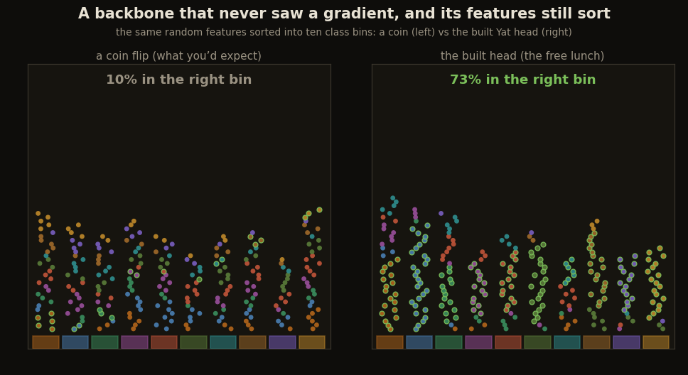
What happens if the backbone never trains at all? That is the cleanest version of the claim, so run it first. Take a backbone with random weights, never trained, and build the head on the garbage features that come out. You would expect nothing, and the trained linear head on those features confirms it: it sits at chance. But the constructed head sorts them anyway.

rnd = Net(nnx.Rngs(0))
con_rand = accuracy(build_head(feats(rnd, Xtr), ytr, feats(rnd, Xte)), yte)
print(con_rand)   # 72.7%

72.7% from a network that never saw a gradient. Random convolutional features are a known free lunch: even an untuned stack of filters keeps enough class structure for a head that only has to read it.

Train the backbone, compare the heads#

Now the ordinary training loop, but on the backbone only. Flax NNX makes the step a few lines: a loss, its gradient, an optimizer update.

net = Net(nnx.Rngs(0)); opt = nnx.Optimizer(net, optax.adam(1e-3), wrt=nnx.Param)

@nnx.jit
def step(net, opt, xb, yb):
    def loss(net):
        return optax.softmax_cross_entropy_with_integer_labels(net(xb), yb).mean()
    l, g = nnx.value_and_grad(loss)(net); opt.update(net, g); return l

for ep in range(6):
    perm = np.random.RandomState(ep).permutation(len(Xtr))
    for i in range(0, len(Xtr) - 256, 256):
        j = perm[i:i + 256]; step(net, opt, Xtr[j], jnp.asarray(ytr[j]))

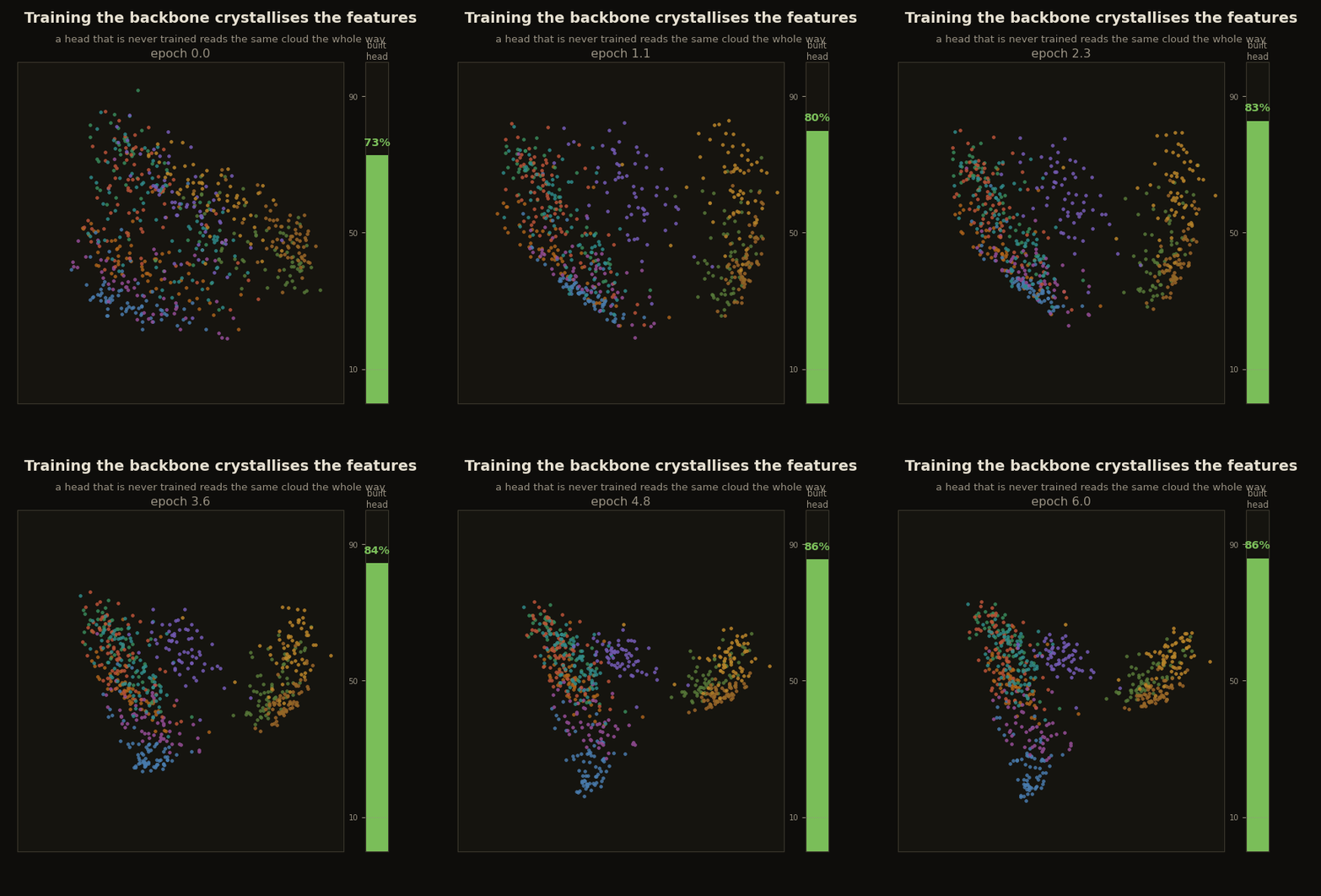
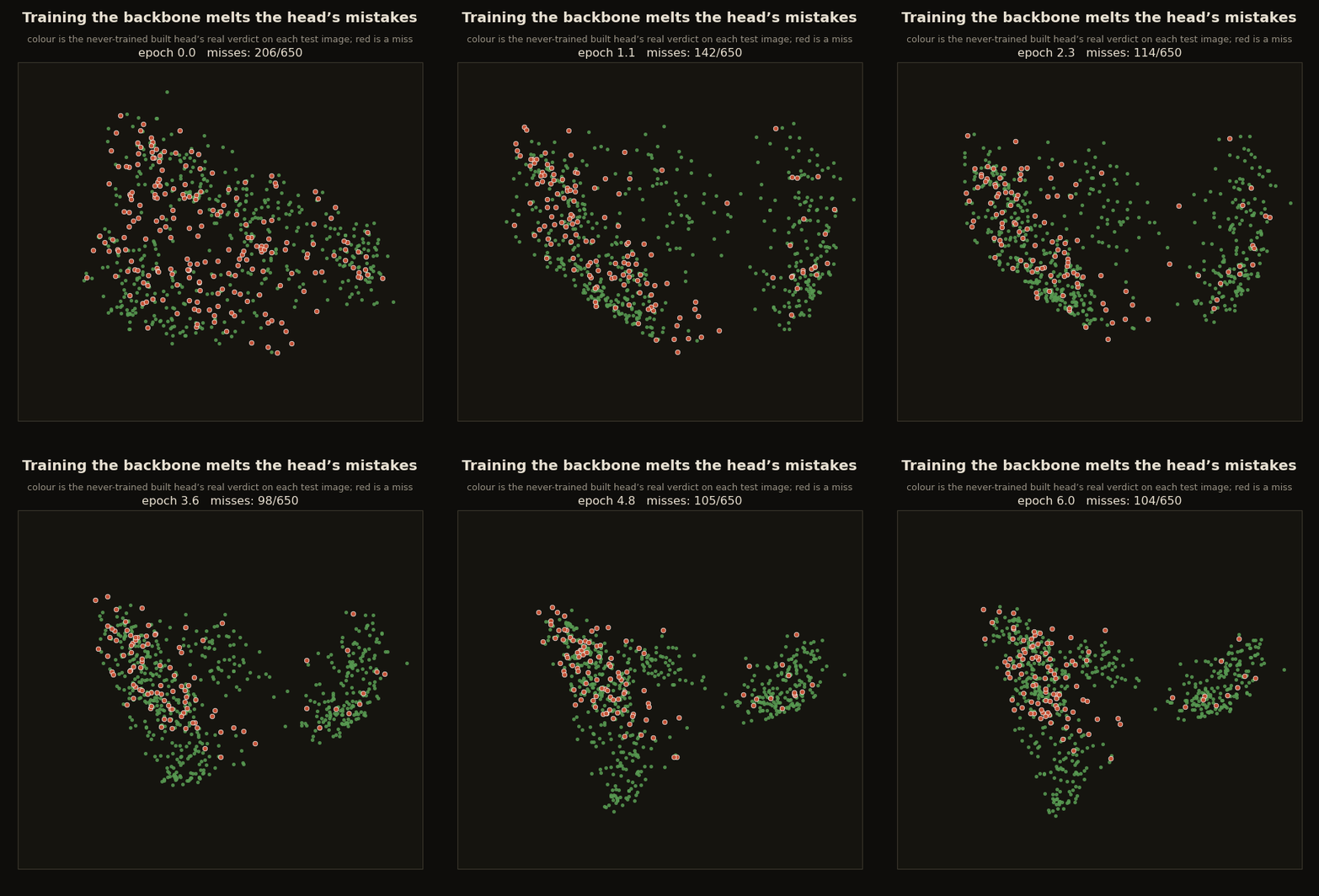
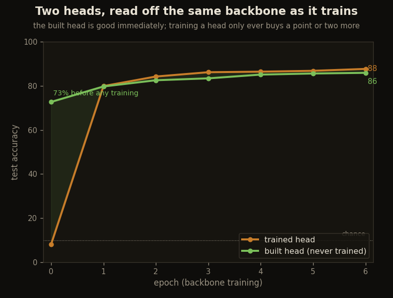
After six epochs the trained head reaches 87.7%. Freeze the same backbone, throw the trained head away, and build a fresh Yat head on its features: 85.9%, with no head training at all. Training the classifier bought under two points; the other seventy-five came from the backbone.

trained = accuracy(net, Xte, yte)                       # 87.7%
con = accuracy(build_head(feats(net, Xtr), ytr, feats(net, Xte)), yte)   # 85.9%

So the curve runs from 72.7% on random features to 85.9% on trained ones, all read by a head that was never trained, always a point or two under the trained head and never more. (The explainer’s 74 / 83.2 / 85.7 are from its reference run, a PyTorch pipeline; the numbers on this page are this post’s own JAX run. The story is identical, the last digits move with the framework and the seed.) The accuracy lives in the representation. The classifier, and its edits, are furniture you place.

The strength of random convolutional features is from Saxe et al. (2011); the prototype head from Chen et al. (2019); Fashion-MNIST from Xiao et al. (2017); the Yat kernel from Bouhsine (2026). The conceptual companion is On Fashion-MNIST, the Head Can Be Built by Hand.

Remove the trained backbone#

The second construction replaces the NNX backbone with a stateless JAX function. Two fixed Sobel kernels produce horizontal and vertical gradients; six angular bins plus one corner channel form the feature bank:

NB, GRID = 6, 7
CENTERS = jnp.linspace(0, jnp.pi, NB, endpoint=False)

@jax.jit
def handbuilt_features(imgs):
    gx, gy = conv3x3(imgs, SX), conv3x3(imgs, SY)
    mag = jnp.sqrt(gx**2 + gy**2) + 1e-6
    ang = jnp.mod(jnp.arctan2(gy, gx), jnp.pi)
    dist = jnp.abs(jnp.mod(ang[:, None] - CENTERS[None, :, None, None]
                           + jnp.pi / 2, jnp.pi) - jnp.pi / 2)
    edges = jnp.clip(1 - dist / (jnp.pi / NB), 0, 1) * mag[:, None]
    corner = (jnp.abs(gx) * jnp.abs(gy))[:, None]
    chans = jnp.concatenate([edges, corner], axis=1)
    pooled = chans.reshape(len(imgs), 7, 7, 4, 7, 4).mean((3, 5))
    z = pooled.reshape(len(imgs), 343)
    return z / (jnp.linalg.norm(z, axis=1, keepdims=True) + 1e-6)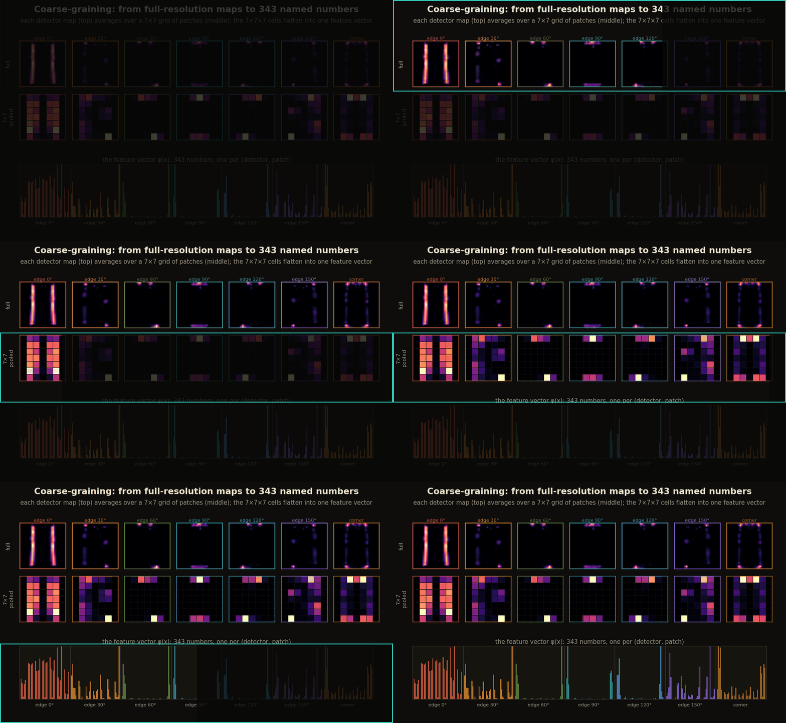

Run class-conditioned k-means on those features, store twenty centers per class, and score each class by its strongest Yat-kernel match. K-means estimates prototype locations from labeled class subsets, so the system is zero-gradient rather than data-free.

Ftr, Fte = np.asarray(handbuilt_features(Xtr)), np.asarray(handbuilt_features(Xte))
W, labels = fit_classwise_kmeans(Ftr, ytr, per_class=20)
scores = yat_kernel(jnp.asarray(Fte), jnp.asarray(W), b=0.5, eps=eps)
pred = np.stack([np.max(scores[:, labels == c], axis=1) for c in range(10)], axis=1).argmax(1)
print(100 * np.mean(pred == yte))  # 83.3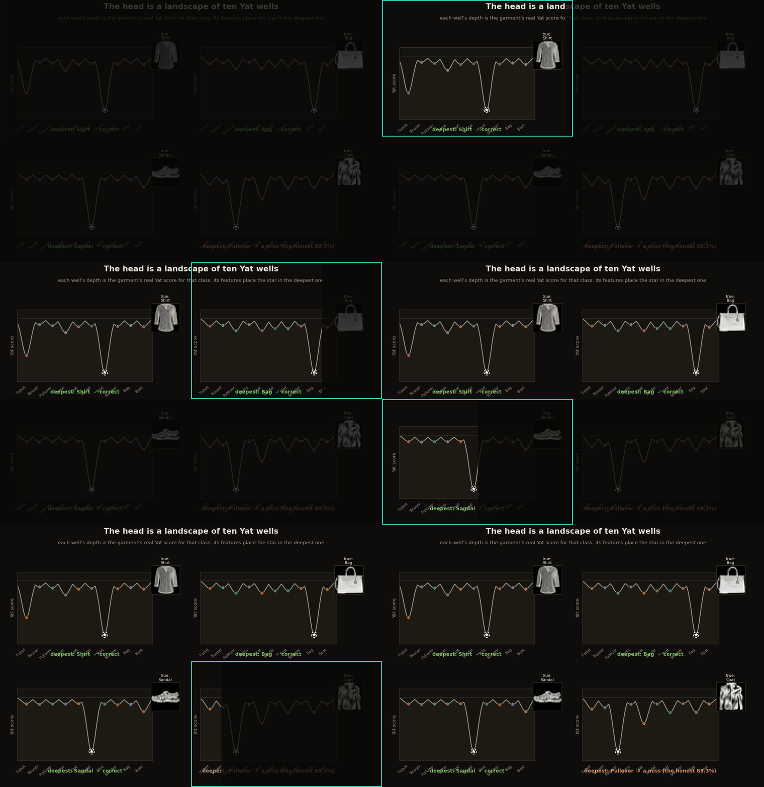

The combined file now contains both comparisons: a constructed head on random and learned backbone features, and a fully hand-built feature extractor with the same prototype logic. The latter reaches 83.3% on this Fashion-MNIST setup; it does not imply that fixed edges transfer to datasets whose useful statistics are not dominated by garment contours.

@misc{bouhsine2026trainthefeaturesjaxflaxnnx,
  author       = {Bouhsine, Taha},
  title        = {Constructing the Fashion-MNIST Network, in JAX/Flax NNX},
  year         = {2026},
  month        = {jun},
  howpublished = {\url{https://tahabouhsine.com/blog/train-the-features-jax-flax-nnx/}},
  note         = {Blog post, Records of the !mmortal Data Scientist}
}