Mixture of Experts

Route each input to a handful of specialist sub-networks with a learnable gate, and keep those specialists busy with a load-balancing loss.

Prerequisites

You should be comfortable training a classifier — see Tabular Data with MLPs — and be able to write your own Custom Training Loops. The residual block structure mirrors the feed-forward layer in a Simple Transformer.

What you'll learn

• Why conditional computation lets you grow model capacity without growing per-input FLOPs
• Implement a MoELayer with a linear gate, jax.lax.top_k routing, and an nnx.List of expert MLPs
• Combine the chosen experts' outputs with a masked einsum
• Add a load-balancing auxiliary loss so the gate can't collapse onto one expert
• Return the auxiliary loss and expert utilization through has_aux and read the routing histogram

Example Code

See the full implementation: examples/scientific/moe.py

Why mixture of experts?

A dense network runs every parameter on every input. If you want more capacity, you pay for it on every forward pass. Mixture of Experts (MoE) breaks that link: you keep a pool of $E$ expert sub-networks but a lightweight gate activates only $k \ll E$ of them per input. Capacity scales with $E$; compute scales with $k$. This is the trick behind the largest sparse language models, where MoE feed-forward layers replace the dense FFN inside each transformer block.

The intuition is specialization. Different regions of input space have different structure — different classes, different regimes, different languages. Rather than force one network to model all of them, the gate learns a soft partition and lets each expert become good at its slice.

We demonstrate this on a synthetic Gaussian-mixture classification task: several well-separated blobs, each its own class. That piecewise structure is exactly what a set of experts can carve up.

The math: top-k routing

Given an input representation $x \in \mathbb{R}^{d}$, a linear gate produces one logit per expert:

$$g = W_g\, x \in \mathbb{R}^{E}$$

We keep only the $k$ largest logits. Let $\mathcal{T}(x)$ be the set of top-$k$ expert indices. The combine weights are a softmax taken over just those $k$ logits:

$$p_e = \frac{\exp(g_e)}{\sum_{j \in \mathcal{T}(x)} \exp(g_j)} \quad\text{for } e \in \mathcal{T}(x), \qquad p_e = 0 \text{ otherwise.}$$

The layer output is the weighted sum of the selected experts' outputs (all other experts contribute nothing):

$$y = \sum_{e \in \mathcal{T}(x)} p_e \; \mathrm{Expert}_e(x)$$

Because $p_e = 0$ outside the top-$k$ set, this is genuinely sparse computation — even though, for simplicity on CPU, our code evaluates all experts and masks the rest.

The math: load balancing

Left alone, the gate finds a shortcut: send everything to one strong expert, let the others wither. To prevent that collapse we add an auxiliary load-balancing loss (Switch-Transformer style). For a batch, define per expert $i$:

• $f_i$ — the fraction of routing slots assigned to expert $i$ (there are $B\cdot k$ slots in a batch of $B$),
• $P_i$ — the mean gate probability mass on expert $i$ (from the full softmax over all experts).

Both vectors sum to $1$. The auxiliary loss is their dot product, scaled by $E$:

$$\mathcal{L}_{\text{balance}} = E \sum_{i=1}^{E} f_i \, P_i$$

This is minimized (value $1$) when load is spread uniformly and grows toward $E$ as routing concentrates. Multiplying $f_i$ (a hard count) by $P_i$ (a smooth probability) keeps the term differentiable through the gate. The total objective is the task loss plus a small multiple of the balance term:

$$\mathcal{L} = \mathcal{L}_{\text{task}} + \alpha \, \mathcal{L}_{\text{balance}}, \qquad \alpha = 0.01$$

The MoE layer

The gate is a bias-free nnx.Linear; the experts are independent MLPs held in an nnx.List (a plain Python list would not register as state on Flax 0.12). We run every expert densely, then mask by the top-$k$ selection with two einsums — one to scatter the combine weights onto a dense $(B, E)$ gate matrix, one to blend the expert outputs.

import jax
import jax.numpy as jnp
from flax import nnx
from shared.models import MLP

class MoELayer(nnx.Module):
    def __init__(self, d_model, d_hidden, n_experts, k, *, rngs: nnx.Rngs):
        self.n_experts = n_experts
        self.k = k
        self.gate = nnx.Linear(d_model, n_experts, use_bias=False, rngs=rngs)
        self.experts = nnx.List([                       # nnx.List, not [ ]
            MLP(d_model, d_hidden, d_model, n_layers=2, rngs=rngs)
            for _ in range(n_experts)
        ])

    def __call__(self, x, train: bool = False):
        gate_logits = self.gate(x)                          # (B, E)
        router_probs = jax.nn.softmax(gate_logits, axis=-1) # (B, E) full softmax

        # top-k routing
        top_vals, top_idx = jax.lax.top_k(gate_logits, self.k)  # (B, k)
        top_gates = jax.nn.softmax(top_vals, axis=-1)           # (B, k)
        one_hot = jax.nn.one_hot(top_idx, self.n_experts)       # (B, k, E)
        dense_gates = jnp.einsum("bk,bke->be", top_gates, one_hot)  # (B, E)

        # run every expert, then combine the selected ones
        expert_out = jnp.stack(
            [expert(x, train=train) for expert in self.experts], axis=1
        )                                                       # (B, E, d_model)
        y = jnp.einsum("be,bed->bd", dense_gates, expert_out)   # (B, d_model)

        # load-balancing statistics
        selection = one_hot.sum(axis=1)                         # (B, E) in {0,1}
        f = selection.sum(axis=0) / (x.shape[0] * self.k)       # (E,) sums to 1
        p = router_probs.mean(axis=0)                           # (E,) sums to 1
        balance_loss = self.n_experts * jnp.sum(f * p)          # =1 when uniform

        return y, balance_loss, f

jax.lax.top_k returns integer indices (no gradient), but the combine weights flow through top_gates = softmax(top_vals), so the gate is trained end-to-end. Experts that aren't selected are multiplied by zero and receive no gradient for that input.

The classifier

We wrap the MoE layer transformer-style: a stem projects the input, a residual connection wraps the MoE block, a LayerNorm stabilizes it, and a linear head produces class logits. The forward pass threads the balance loss and utilization back out alongside the logits.

class MoEClassifier(nnx.Module):
    def __init__(self, in_features, d_model, d_hidden, n_experts, k, n_classes, *, rngs):
        self.stem = nnx.Linear(in_features, d_model, rngs=rngs)
        self.moe = MoELayer(d_model, d_hidden, n_experts, k, rngs=rngs)
        self.norm = nnx.LayerNorm(d_model, rngs=rngs)
        self.head = nnx.Linear(d_model, n_classes, rngs=rngs)

    def __call__(self, x, train: bool = False):
        h = nnx.relu(self.stem(x))                  # (B, d_model)
        moe_out, balance_loss, util = self.moe(h, train=train)
        h = self.norm(h + moe_out)                  # residual around the MoE block
        logits = self.head(h)                       # (B, n_classes)
        return logits, balance_loss, util

model = MoEClassifier(32, 64, 128, n_experts=4, k=2, n_classes=6, rngs=nnx.Rngs(0))

The train step

The total loss is task cross-entropy plus a small multiple of the balance loss. Because the model returns three things, we bundle the extras into the has_aux tuple so nnx.value_and_grad differentiates only the scalar total:

import optax

AUX_COEF = 0.01

@nnx.jit
def train_step(model, optimizer, batch):
    def loss_fn(model):
        logits, balance_loss, util = model(batch["x"], train=True)
        ce = optax.softmax_cross_entropy_with_integer_labels(logits, batch["y"]).mean()
        total = ce + AUX_COEF * balance_loss
        return total, (ce, balance_loss, util)

    (total, (ce, balance_loss, util)), grads = nnx.value_and_grad(loss_fn, has_aux=True)(model)
    optimizer.update(model, grads)
    return total, ce, balance_loss, util

optimizer = nnx.Optimizer(model, optax.adam(3e-3), wrt=nnx.Param)
for step in range(300):
    total, ce, bal, util = train_step(model, optimizer, batch)

Results / What to expect

Training a top-2-of-4 MoE on the synthetic 6-class mixture takes a few seconds on CPU. Task cross-entropy collapses toward zero and accuracy hits 100%, while the balance loss hovers near its floor of $1.0$ — the sign of an evenly loaded gate:

$ python scientific/moe.py
Training a top-2-of-4 MoE classifier for 300 steps (6 classes, batch 512)

step    0 | total 2.2347 | ce 2.2194 | balance 1.532 | acc 0.646
step   50 | total 0.0107 | ce 0.0007 | balance 0.999 | acc 1.000
step  100 | total 0.0103 | ce 0.0004 | balance 0.991 | acc 1.000
step  150 | total 0.0102 | ce 0.0003 | balance 0.989 | acc 1.000
step  200 | total 0.0102 | ce 0.0003 | balance 0.988 | acc 1.000
step  250 | total 0.0101 | ce 0.0002 | balance 0.985 | acc 1.000
step  299 | total 0.0100 | ce 0.0002 | balance 0.983 | acc 1.000

Final expert utilization (fraction of routing slots):
  e0:0.26  e1:0.23  e2:0.26  e3:0.25

The utilization histogram is the diagnostic to watch: each expert handles roughly $1/E = 0.25$ of the routing slots. The script saves this histogram as a bar chart at the end of training:

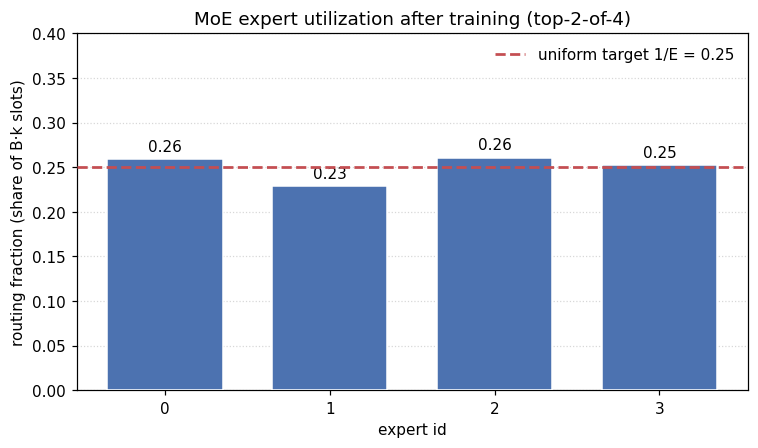
Each bar is the fraction of the batch's $B\cdot k$ routing slots sent to that expert; the dashed line marks the uniform $1/E = 0.25$ target. All four bars land right on the line — the load-balancing loss did its job, and no expert went dead.

If you drop AUX_COEF to 0.0, the same run tends to concentrate mass on one or two experts (utilization like e0:0.5 e1:0.4 e2:0.05 e3:0.05) — capacity you paid for but never use.

Common pitfalls

Plain Python list of experts.

❌ A bare list won't register as state and crashes on Flax 0.12.

self.experts = [MLP(...) for _ in range(n_experts)]

✅ Wrap the expert collection in nnx.List.

self.experts = nnx.List([MLP(...) for _ in range(n_experts)])

No load-balancing loss.

❌ Task loss alone lets the gate collapse onto one expert; the rest go dead.

total = ce                                  # gate collapses over time

✅ Add the balance term so usage stays spread out.

total = ce + AUX_COEF * balance_loss

Softmaxing over all experts for the combine weights.

❌ A full softmax leaks probability mass onto experts you didn't select.

weights = jax.nn.softmax(gate_logits, axis=-1)   # (B, E) — not sparse

✅ Softmax over the top-k logits only, then scatter back.

top_vals, top_idx = jax.lax.top_k(gate_logits, k)
top_gates = jax.nn.softmax(top_vals, axis=-1)    # (B, k)

Trying to backprop through the routing indices.

❌ top_idx is integer-valued and has no gradient — routing there is a no-op.

loss = something(top_idx)                   # gate never learns

✅ Let gradients flow through the softmax weights, not the indices.

y = jnp.einsum("be,bed->bd", dense_gates, expert_out)   # dense_gates carries grad

A huge AUX_COEF.

❌ Over-weighting balance forces perfectly uniform routing and kills specialization.

total = ce + 1.0 * balance_loss             # gate ignores the input

✅ Keep it small (≈0.01) — a nudge, not the objective.

total = ce + 0.01 * balance_loss

Next steps

• Neural ODEs — another way to add capacity through structure rather than raw width.
• GPT from scratch — where MoE layers replace the dense FFN inside each transformer block at scale.

Complete Example

examples/scientific/moe.py — the full, runnable MoE classifier: gate, top-k routing, nnx.List of expert MLPs, load-balancing loss, and the utilization readout.

References

• Shazeer et al. (2017), Outrageously Large Neural Networks: The Sparsely-Gated Mixture-of-Experts Layer — arXiv:1701.06538
• Fedus, Zoph & Shazeer (2021), Switch Transformers: Scaling to Trillion Parameter Models with Simple and Efficient Sparsity — arXiv:2101.03961
• Lepikhin et al. (2020), GShard: Scaling Giant Models with Conditional Computation and Automatic Sharding — arXiv:2006.16668
• Zoph et al. (2022), ST-MoE: Designing Stable and Transferable Sparse Expert Models — arXiv:2202.08906