Physics-Informed Neural Networks (PINNs)

Solve a differential equation with a neural network — and not a single training label in sight. The equation is the supervision.

Prerequisites

You should be comfortable building a model (your first model) and writing your own loop (custom training loops, training best practices). A little calculus (derivatives, second-order ODEs) helps.

What you'll learn

• How a PINN turns a differential equation into a loss function with no dataset
• How to differentiate the network's output with respect to its input using jax.grad — twice
• Why jax.grad(jax.grad(...)) plus vmap is the perfect tool for this
• Why smooth activations (tanh, not ReLU) are non-negotiable for second-order physics
• How to enforce initial conditions so the network learns the right solution

Example Code

See the full implementation: examples/scientific/pinn_oscillator.py

This guide is different

Every other guide on this site fits a model to data: you have inputs x, targets y, and a loss that measures the gap. Here there is no y. Instead you have a law of physics the solution must obey, and you turn that into the loss.

The trick is that a neural network $\hat u_\theta(t)$ is a smooth, differentiable function of its input. So we can ask JAX for its derivatives with respect to the input $t$ and check whether they satisfy the governing equation. This is the one guide where you differentiate the model itself, not a loss over samples.

The problem: a damped harmonic oscillator

A mass on a spring with friction obeys a second-order linear ODE:

$$u''(t) + 2\zeta\omega\, u'(t) + \omega^2 u(t) = 0, \qquad u(0) = 1,\ \ u'(0) = 0,$$

on $t \in [0, T]$, where $\omega$ is the natural frequency and $\zeta$ the damping ratio. For the underdamped case ($0 < \zeta < 1$) the exact solution is a decaying cosine, which we only use to check our network afterward:

$$u(t) = e^{-\zeta\omega t}\left(\cos(\omega_d t) + \frac{\zeta\omega}{\omega_d}\sin(\omega_d t)\right), \qquad \omega_d = \omega\sqrt{1 - \zeta^2}.$$

From equation to loss

Let $\hat u_\theta(t)$ be our network. Define the residual — how badly the network violates the ODE at a point $t$:

$$r_\theta(t) = \hat u_\theta''(t) + 2\zeta\omega\, \hat u_\theta'(t) + \omega^2 \hat u_\theta(t).$$

If $\hat u_\theta$ were the true solution, $r_\theta(t) = 0$ everywhere. So we sample a set of collocation points $\{t_i\}_{i=1}^N$ on $[0, T]$ (just a linspace — no dataset) and minimize the mean-squared residual, plus a penalty pinning down the initial conditions:

$$\mathcal{L}(\theta) = \underbrace{\frac{1}{N}\sum_{i=1}^N r_\theta(t_i)^2}_{\text{physics}} \;+\; \lambda\,\underbrace{\big[(\hat u_\theta(0) - 1)^2 + \hat u_\theta'(0)^2\big]}_{\text{initial conditions}}.$$

The initial-condition term is not optional. The trivial function $u \equiv 0$ also satisfies the ODE — the IC penalty is what forces the network onto the one solution we want.

The derivatives $\hat u_\theta'$ and $\hat u_\theta''$ are computed exactly by automatic differentiation, not finite differences. jax.grad gives $\hat u_\theta'$, and jax.grad again gives $\hat u_\theta''$. This is why JAX is ideal for PINNs: you can differentiate through the network with respect to its input, arbitrarily many times, and compose that with vmap (evaluate at all collocation points) and jit (compile the whole thing).

The model

A small MLP mapping a scalar $t$ to a scalar $u$. The activation matters: tanh is smooth, so its first and second derivatives are well-behaved — a ReLU network has a zero second derivative almost everywhere, which would make the physics loss meaningless.

import jax
import jax.numpy as jnp
from flax import nnx
import optax

OMEGA = 3.0    # natural frequency
ZETA = 0.2     # damping ratio (0 < zeta < 1)
T = 4.0        # domain [0, T]
W_IC = 10.0    # weight on the initial-condition term


class PINN(nnx.Module):
    """Scalar-in, scalar-out MLP approximating u(t)."""

    def __init__(self, hidden: int = 32, n_layers: int = 4, *, rngs: nnx.Rngs):
        layers = [nnx.Linear(1, hidden, rngs=rngs)]
        for _ in range(n_layers - 1):
            layers.append(nnx.Linear(hidden, hidden, rngs=rngs))
        self.layers = nnx.List(layers)          # nnx.List, not a plain list!
        self.out = nnx.Linear(hidden, 1, rngs=rngs)

    def __call__(self, t):
        x = t
        for layer in self.layers:
            x = nnx.tanh(layer(x))
        return self.out(x)

The physics loss

This is the heart of the method. We define a scalar helper u_fn(t) and differentiate it with respect to t — twice — then vmap the derivatives over every collocation point:

def physics_loss(model, t_coll):
    def u_fn(t):                    # scalar t -> scalar u(t)
        return model(t.reshape(1, 1))[0, 0]

    u_t_fn = jax.grad(u_fn)         # du/dt   via autodiff
    u_tt_fn = jax.grad(u_t_fn)      # d2u/dt2 via autodiff-of-autodiff

    t_flat = t_coll[:, 0]
    u = jax.vmap(u_fn)(t_flat)
    u_t = jax.vmap(u_t_fn)(t_flat)
    u_tt = jax.vmap(u_tt_fn)(t_flat)

    residual = u_tt + 2.0 * ZETA * OMEGA * u_t + OMEGA ** 2 * u
    loss_res = jnp.mean(residual ** 2)

    # Initial conditions u(0)=1, u'(0)=0 as a soft penalty.
    t0 = jnp.array(0.0)
    loss_ic = (u_fn(t0) - 1.0) ** 2 + (u_t_fn(t0) - 0.0) ** 2

    total = loss_res + W_IC * loss_ic
    return total, {"residual": loss_res, "ic": loss_ic}

Note the elegant separation of concerns: the inner jax.grad calls differentiate with respect to the input t (the network weights are held fixed there), while the outer nnx.value_and_grad in the train step differentiates the whole loss with respect to the parameters. JAX composes these nested derivatives for you.

The training step

Standard NNX training step — the only unusual thing is that batch is just the array of collocation points, not (x, y) pairs:

@nnx.jit
def train_step(model, optimizer, batch):
    def loss_fn(model):
        total, aux = physics_loss(model, batch)
        return total, aux

    (loss, aux), grads = nnx.value_and_grad(loss_fn, has_aux=True)(model)
    optimizer.update(model, grads)
    return loss, aux

And the driver — the collocation points come from a plain linspace, and Adam does the rest:

rngs = nnx.Rngs(0)
model = PINN(hidden=32, n_layers=4, rngs=rngs)
optimizer = nnx.Optimizer(model, optax.adam(2e-3), wrt=nnx.Param)

t_coll = jnp.linspace(0.0, T, 100).reshape(-1, 1)   # no dataset!

for step in range(3000):
    loss, aux = train_step(model, optimizer, t_coll)

Results / What to expect

On CPU this converges in a couple of seconds. The physics residual and IC penalty both fall by orders of magnitude, and the learned $\hat u(t)$ tracks the analytic damped cosine to within about 0.01 across the whole domain:

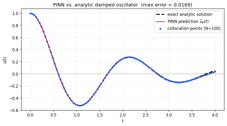
The red PINN curve sits almost exactly on top of the dashed analytic solution across all collocation points (blue) — visual proof that minimizing only the ODE residual plus initial conditions, with no target data, recovered the true trajectory.

$ python scientific/pinn_oscillator.py
Solving u'' + 2*0.2*3.0*u' + 3.0^2*u = 0 on [0, 4.0]
steps=3000  collocation=100

step     0 | loss 1.1635e+01 | residual 5.151e-01 | ic 1.112e+00
step   500 | loss 2.3581e-01 | residual 2.295e-01 | ic 6.289e-04
step  1000 | loss 1.7431e-01 | residual 1.451e-01 | ic 2.919e-03
step  1500 | loss 1.3456e-02 | residual 1.343e-02 | ic 2.544e-06
step  2000 | loss 8.0015e-03 | residual 7.976e-03 | ic 2.577e-06
step  2500 | loss 4.9807e-03 | residual 4.979e-03 | ic 2.122e-07
step  2999 | loss 3.1823e-03 | residual 3.181e-03 | ic 9.729e-08

max |u_pred - u_analytic| over [0, 4.0] = 0.0118

The network never saw the analytic solution during training — it recovered it purely from the differential equation and the two initial conditions.

Run bigger or smaller with environment variables: EPOCHS (optimization steps), BATCH (number of collocation points).

Common Pitfalls

• ❌ ReLU activations. A ReLU MLP is piecewise-linear, so its second derivative is zero almost everywhere and the physics residual becomes garbage. ✅ Use a smooth activation like tanh (or sin, gelu) so u' and u'' are meaningful.

• ❌ Dropping the initial-condition term. The homogeneous ODE is also satisfied by the trivial solution $u \equiv 0$; without an IC penalty the network may happily collapse to it. ✅ Add the IC penalty and weight it (W_IC) so it competes with the residual term.

• ❌ Differentiating the wrong thing. Beginners reach for the parameter gradient when they need the input gradient. ✅ Define a scalar u_fn(t) and jax.grad over t; let the outer nnx.value_and_grad handle the parameters.

• ❌ A plain Python list of layers. self.layers = [ ... ] crashes the pytree machinery on Flax 0.12. ✅ Wrap submodule lists in nnx.List([ ... ]) (and dicts in nnx.Dict).

• ❌ Looping over collocation points in Python. Calling the derivative one point at a time is painfully slow. ✅ jax.vmap the scalar derivative over the whole batch of points at once.

Next steps

• Graph Neural Networks — the other frontier of "new data modalities" in this track.
• Custom training loops — the loop patterns underneath this example.
• Training best practices — for scaling PINNs to stiffer, higher-dimensional PDEs.

Complete Example

examples/scientific/pinn_oscillator.py — a self-contained PINN that solves the damped-oscillator ODE and reports the max error against the analytic solution.

References

• Raissi, Perdikaris, Karniadakis. Physics Informed Deep Learning (Part I): Data-driven Solutions of Nonlinear Partial Differential Equations. arXiv:1711.10561
• Raissi, Perdikaris, Karniadakis. Physics Informed Deep Learning (Part II): Data-driven Discovery of Nonlinear Partial Differential Equations. arXiv:1711.10566
• Baydin, Pearlmutter, Radul, Siskind. Automatic Differentiation in Machine Learning: a Survey. arXiv:1502.05767