Distillation as Kernel Transfer, in JAX/Flax NNX
#ml#knowledge-distillation#dark-knowledge#kernel-methods#jax#flax#nnx#implementation#representation-learning#fashion-mnist
Part 6 of 6Geometry of Representations
- 1What Activations Do to Geometry
- 2Untangling the Moons: A Visual History of Contrastive Learning
- 3What Makes a Good Latent Space? The Welch Bound and the Simplex
- 4Latent on the Spectrum: Why Cats Sit Closer to Dogs Than to Cars
- 5The Three States of Information
- 6Distillation Is a Geometry, Not an Answer Keythis post's explainer
One loss function in this post is the entire experiment. It takes a batch of images, asks the teacher for its softened outputs, turns those into a pairwise Gram, and penalizes the student’s embedding Gram for disagreeing with it. No integer label is ever passed in. Everything else here, the teacher CNN in Flax NNX, the five-line kernel extraction, the two probes, exists to say what a student trained on that loss learned anyway, which the explainer reads as evidence that distillation moves a geometry rather than an answer key.
Prefer a notebook? Run the whole thing on Kaggle: the same code, block by block, with the math written out and every figure reproduced from a real run.
The teacher, an ordinary CNN
Where does dark knowledge come from? From a network that already knows something. So the first thing to build is an ordinary teacher: a small convolutional classifier on Fashion-MNIST, trained the usual way on labels. One design choice does matter downstream. The module exposes its penultimate layer through an embed method, because everything below reads geometry off that latent, never off the logits.
import jax, jax.numpy as jnp, optax
from flax import nnx

class CNN(nnx.Module):
    def __init__(self, c1, c2, d, rngs):
        self.conv1 = nnx.Conv(1, c1, kernel_size=(3, 3), rngs=rngs)
        self.conv2 = nnx.Conv(c1, c2, kernel_size=(3, 3), rngs=rngs)
        self.fc = nnx.Linear(c2 * 7 * 7, d, rngs=rngs)
        self.head = nnx.Linear(d, 10, rngs=rngs)

    def embed(self, x):                       # the latent the probes and Grams read
        x = nnx.relu(self.conv1(x)); x = nnx.max_pool(x, (2, 2), strides=(2, 2))
        x = nnx.relu(self.conv2(x)); x = nnx.max_pool(x, (2, 2), strides=(2, 2))
        return self.fc(x.reshape(x.shape[0], -1))

    def __call__(self, x):
        return self.head(nnx.relu(self.embed(x)))

teacher = CNN(16, 32, 64, nnx.Rngs(0))        # student is the same, thinner: CNN(8, 16, 32)
Trained six epochs with Adam on plain cross-entropy, this teacher reaches 87.2% test accuracy. That is the reference geometry. Nothing about it is special; the point of the experiment is what can be recovered from its outputs alone.
The kernel, extracted in five lines
What does one softened output carry? At temperature , the teacher’s softmax over a garment is a vector of resemblances, and the outer product is one noisy receipt of how the classes relate from where that garment sits. Average the receipts over the test set and the class-similarity kernel falls out:
In code that is a softmax and a mean of outer products, nothing more. The same three lines, swept over a grid of temperatures, give the whole story of how much geometry the outputs leak.
def class_kernel(z, T):                        # z: [N, 10] teacher test logits
    p = jax.nn.softmax(z / T, axis=1)
    S = (p[:, :, None] * p[:, None, :]).mean(0)  # E[p pᵀ], a 10x10 kernel
    d = jnp.sqrt(jnp.diag(S))
    return S / jnp.outer(d, d)                  # diagonal-normalized to unit self-similarity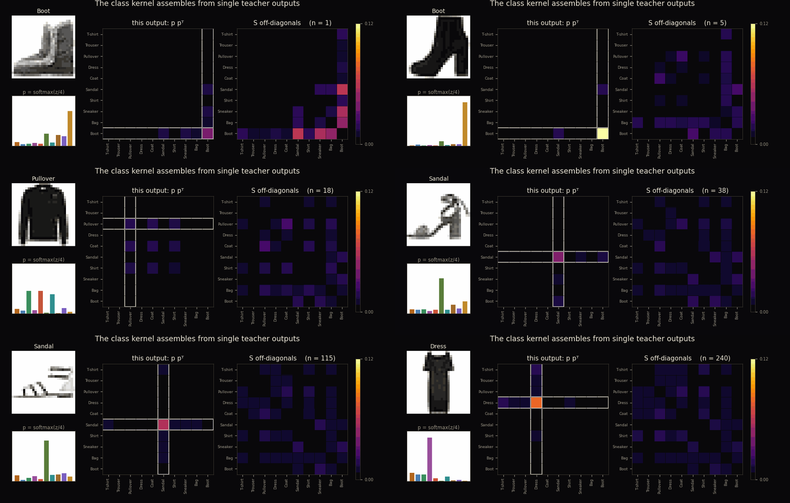
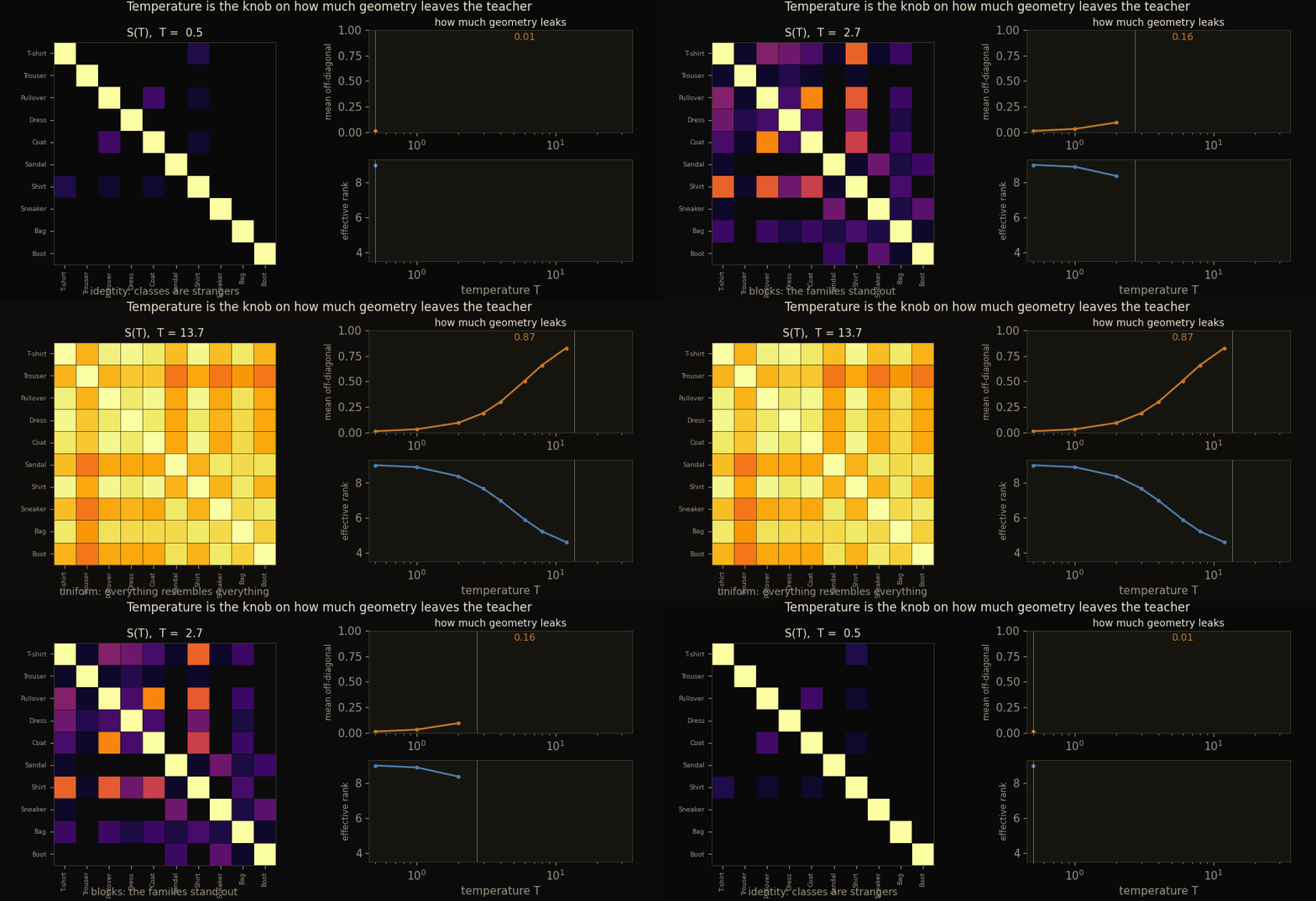
Read across the temperature grid, the kernel’s mean off-diagonal climbs from 0.032 at through 0.298 at to 0.902 at , and its effective rank falls from 8.9 to 7.0 to 4.3. Cold, the classes are strangers and is near the identity; hot, everything resembles everything and washes toward uniform. The choice selects a specific geometry in between, and everything the student inherits is downstream of it.
The standard-KD student, for reference
Before stripping distillation to the kernel, it helps to have the ordinary version in the same code. Classic distillation matches the student’s softened output to the teacher’s soft targets by a KL divergence at temperature , with the usual scaling so the gradient magnitude survives the softening. No hard labels enter, but the per-class structure of the teacher’s output does: the student is still told, class by class, what the answer should look like.
@nnx.jit
def step_kd(model, opt, x, p_t):               # p_t: teacher soft targets at T
    def loss_fn(m):
        logq = jax.nn.log_softmax(m(x) / TEMP)
        return (TEMP ** 2) * (p_t * (jnp.log(p_t + 1e-12) - logq)).sum(1).mean()
    loss, grads = nnx.value_and_grad(loss_fn)(model)
    opt.update(model, grads)
    return loss
The KD student reaches 84.6% direct accuracy, 85.8% linear-probe. On a small, clean dataset with abundant labels, soft targets have little to add over the labels themselves, so this baseline does not beat the label-trained student. That is expected, and beside the point. The question is not whether distillation wins; it is what distillation moves.
The kernel-only student, where no label appears
Here is the loss the whole experiment turns on. Strip away the labels, the soft targets, even the teacher’s head. For each batch, the teacher’s softened outputs define a cosine similarity for every pair of examples, and the student’s only job is to make its embedding geometry reproduce that Gram. The loss never mentions a class; it only ever says these two should be this similar.
@nnx.jit
def step_kernel(model, opt, x, pn):            # pn: L2-normalized teacher soft outputs
    def loss_fn(m):
        g_t = pn @ pn.T                        # teacher's target Gram for this batch
        e = m.embed(x)
        en = e / (jnp.linalg.norm(e, axis=1, keepdims=True) + 1e-8)
        g_s = en @ en.T                        # student's embedding Gram
        mask = 1.0 - jnp.eye(x.shape[0])       # off-diagonal only: relations, not norms
        return (((g_s - g_t) ** 2) * mask).sum() / mask.sum()
    loss, grads = nnx.value_and_grad(loss_fn)(model)
    opt.update(model, grads)
    return loss
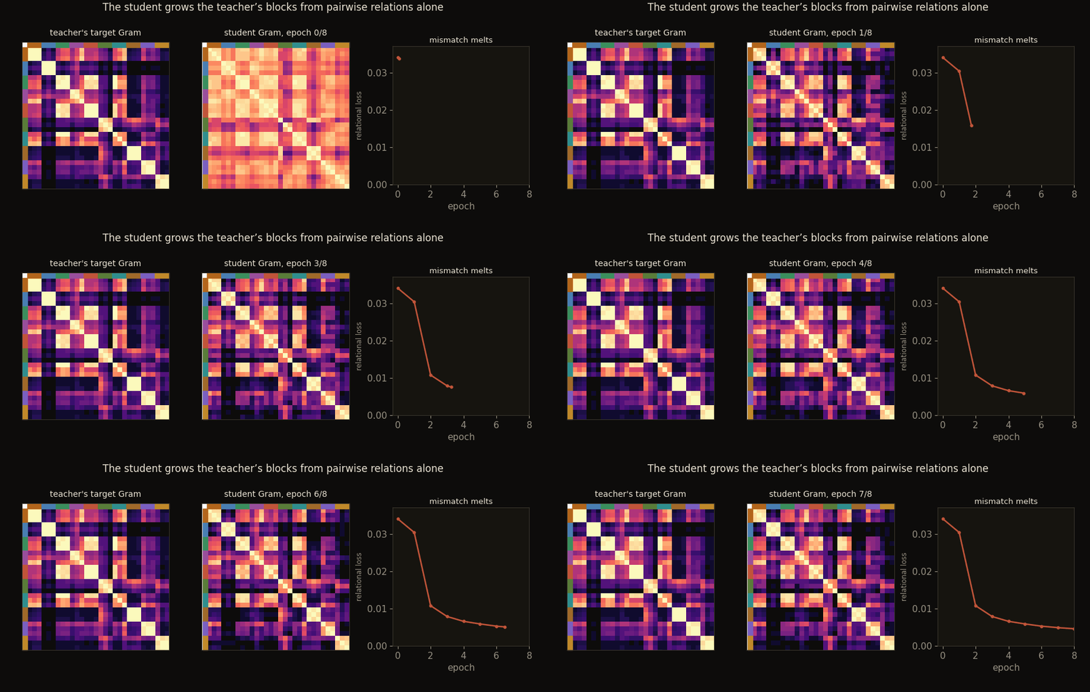
There is no classifier head in this student’s training path at all. The teacher’s soft outputs enter only as pn, a Gram target; no integer label is ever passed. Watch the geometry cross the wire: the student’s batch Gram over thirty held-out garments, checkpointed every epoch, develops the teacher’s block structure while the relational loss melts.
Measuring everyone the same way
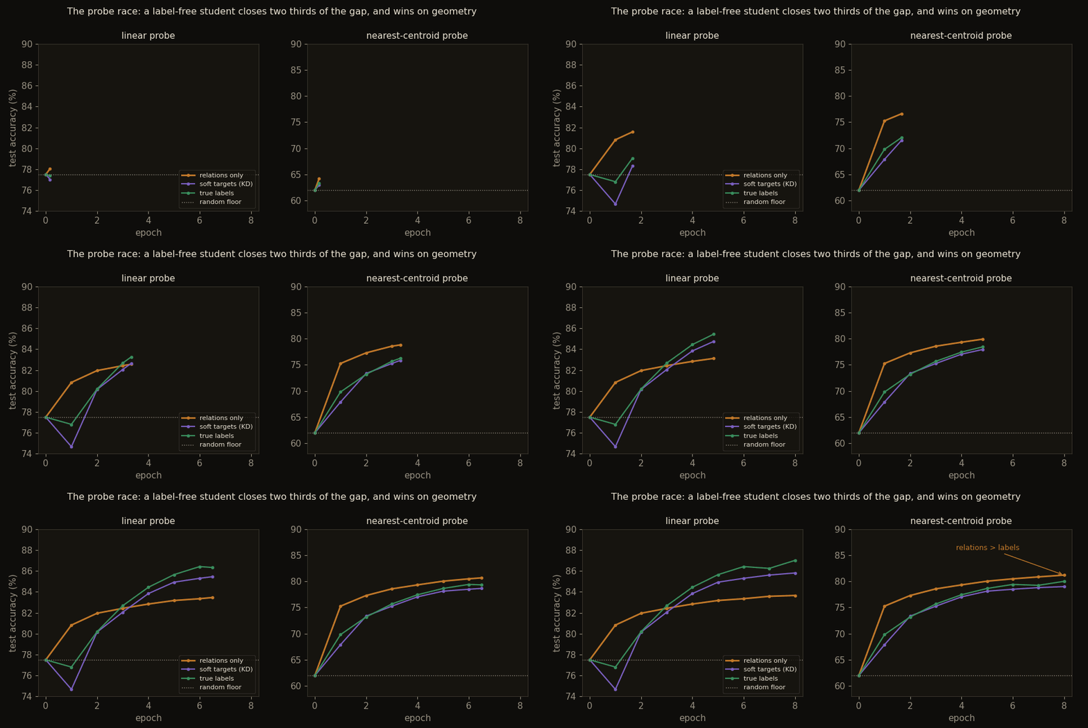
Since the relational student has no head, competence has to be read off its frozen embedding, and the fairest thing is to read every model’s embedding the same way. Two probes, and labels enter only here, in the ruler, never in the student’s gradient. A linear probe is allowed to shear and re-weight the space to find the classes; a nearest-centroid probe is not allowed to fix anything, so it only succeeds if the classes already sit in tight, well-placed clumps.
from sklearn.linear_model import LogisticRegression

def probes(model, Xtr, ytr, Xte, yte):
    Etr, Ete = embed_of(model, Xtr), embed_of(model, Xte)   # frozen latents
    linear = 100.0 * LogisticRegression(max_iter=1000).fit(Etr, ytr).score(Ete, yte)
    mu = np.stack([unit(Etr)[ytr == c].mean(0) for c in range(10)])   # class centroids
    pred = (unit(Ete) @ unit(mu).T).argmax(1)               # nearest centroid, no weights
    return linear, 100.0 * (pred == yte).mean()
The five runs, from the run (relational student across seeds 0, 1, 2; everything else seed 0):
| run | training signal | linear probe | nearest centroid |
|---|---|---|---|
| teacher | labels | 88.1% | 81.7% |
| soft targets (KD) | teacher’s | 85.8% | 79.0% |
| relations only | pairwise similarities | 83.7 / 84.5 / 84.9% | 81.2 / 81.0 / 81.4% |
| true labels | the answer key | 87.0% | 80.0% |
| random init | nothing | 77.5% | 62.0% |
The floor is high: a random CNN already probes at 77.5% linear, so nobody gets credit for the first three-quarters of the scale. The interval that measures training runs from 77.5 to the label ceiling at 87.0, and the relations-only student lands at 83.7 to 84.9, about two-thirds of what a label could add, from a signal that never contained a label. And on the ruler that cannot cheat, the nearest-centroid probe, the label-free student scores 81.2%, above the label-trained student’s 80.0% and essentially at the teacher’s own 81.7%.
Whose spectrum, and whose mistakes
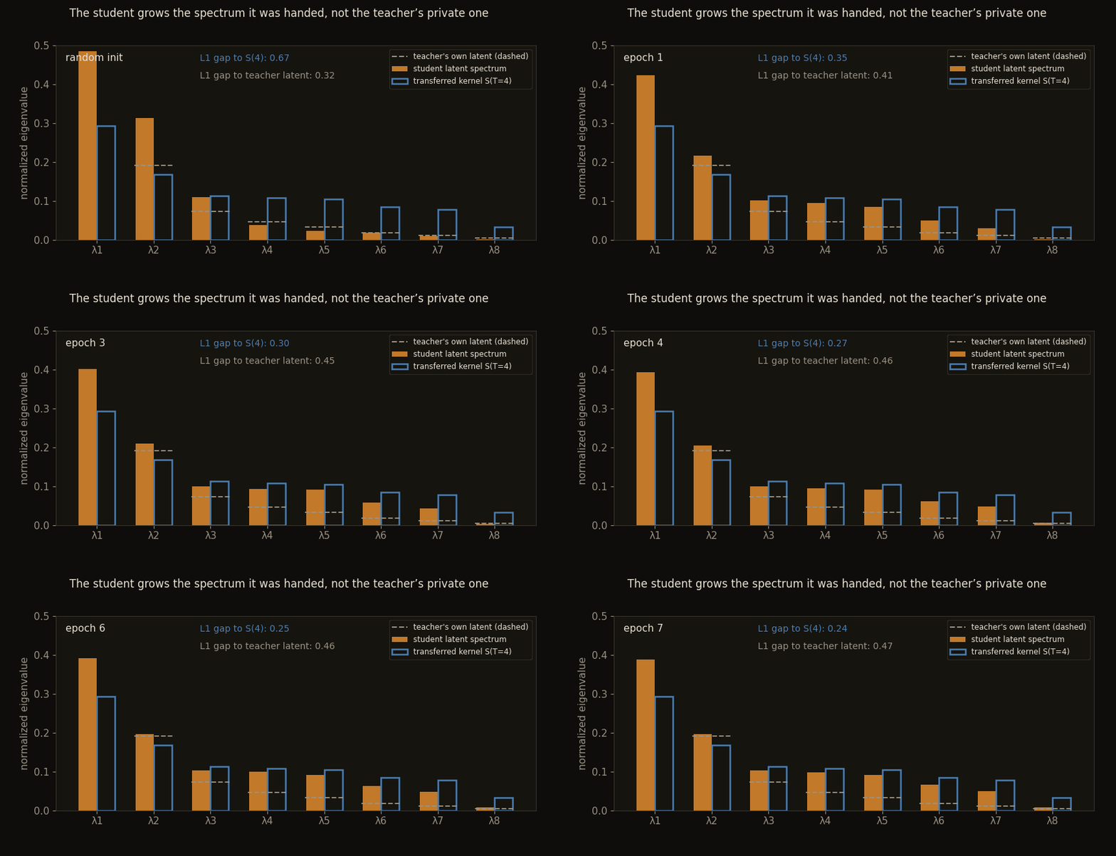
If a latent space is the spectral embedding of a class kernel, then a student trained on a kernel should not merely probe well; its latent geometry should become that kernel’s, eigenvalue by eigenvalue. Two candidate kernels sit in the experiment: the teacher’s own private latent geometry, and , the version of it that went through the softmax and out onto the wire. They are not the same object, and the student inherits the one that was actually handed over.
def spectrum(G):                               # normalized eigenvalue profile of a 10x10 Gram
    w = np.clip(np.linalg.eigvalsh(G)[::-1], 0, None)
    return w / (w.sum() + 1e-12)
Measured, the copy is more faithful to the wire than the author is. By the last epoch the student’s class-mean Gram agrees with at CKA 0.976, while the teacher’s own latent Gram agrees with it at only 0.854. In L1 spectrum distance the student sits at 0.24 from the transferred kernel but 0.47 from the teacher’s private latent; the KD and label students, which fit answers rather than relations, stay close to the teacher-latent shape instead (L1 0.06 and 0.03).
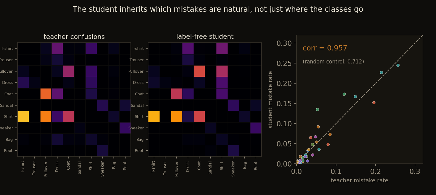
The inherited geometry even fails like the teacher. Rank every model’s off-diagonal confusions on the test set and the relational student’s mistake pattern correlates with the teacher’s at 0.957 (the random control manages 0.712). The teacher’s centroid probe sends stray Shirts mostly to T-shirt, Pullover, and Coat at rates 0.26, 0.22, 0.15; the label-free student’s rates are 0.24, 0.23, 0.17. It did not just learn where the classes are; it learned which mistakes are natural.
What the code shows
The whole experiment is one script and five networks. The teacher serializes its class kernel through its softened outputs; a student that matches nothing but pairwise relations reconstructs the embedding on its side of the wire, closes about two-thirds of the random-to-labels gap, out-organizes the label-trained student on the geometry-native probe, and grows the transferred kernel’s spectrum eigenvalue by eigenvalue. None of the numbers here are chosen. They are what the run prints, and the loss that produced the label-free student never once named a class.
Relational distillation as a method is the RKD / similarity-preserving line (Park et al., 2019; Tung and Mori, 2019); CKA is from Kornblith et al. (2019); the dark-knowledge puzzle from Hinton et al. (2015); Fashion-MNIST from Xiao et al. (2017). The conceptual companion is Distillation Is a Geometry, Not an Answer Key.
Cite as
Bouhsine, T. (). Distillation as Kernel Transfer, in JAX/Flax NNX. Records of the !mmortal Data Scientist. https://tahabouhsine.com/blog/distillation-is-kernel-transfer-jax-flax-nnx/
BibTeX
@misc{bouhsine2026distillationiskerneltransferjaxflaxnnx,
  author       = {Bouhsine, Taha},
  title        = {Distillation as Kernel Transfer, in JAX/Flax NNX},
  year         = {2026},
  month        = {jul},
  howpublished = {\url{https://tahabouhsine.com/blog/distillation-is-kernel-transfer-jax-flax-nnx/}},
  note         = {Blog post, Records of the !mmortal Data Scientist}
}References
- (2015). Distilling the Knowledge in a Neural Network. arXiv:1503.02531
- (2019). Relational Knowledge Distillation. CVPR 2019.arXiv:1904.05068
- (2019). Similarity-Preserving Knowledge Distillation. ICCV 2019.arXiv:1907.09682
- (2019). Similarity of Neural Network Representations Revisited. ICML 2019.arXiv:1905.00414
- (2017). Fashion-MNIST: a Novel Image Dataset for Benchmarking Machine Learning Algorithms. arXiv:1708.07747