Measuring Attention's Geometry in JAX/Flax NNX

July 19, 2026 · 9 min read

#attention #kernels #geometry #jax #flax #nnx #implementation

Part 6 of 6Attention Is a Kernel

Explainer companionThe Geometry of Attention Is a Choice of KernelWant the full intuition first? This is the runnable companion to the explainer.Read the explainer

The explainer derives the territory maps of the two attention laws and then checks the theorems on trained transformers. This is the measurement side: the telemetry that exports a trained head’s real query and key vectors, the offline replays that recompute winners under rescaled queries, the hull linear program, and the census. The models and training harness are scripts/yat_attention.py, the same script the kernel-attention contest ran; the analysis is scripts/export_attention_geometry_viz.py; figures are rendered from the bundles by scripts/render_attention_geometry_gifs.py. Bundles: kgl_blog-attngeom-qk and kgl_blog-attngeom-goat.

Exporting the geometry

Everything in the explainer’s measured half rides on one small addition to the attention module: alongside the maps, the telemetry can now capture the actual projected vectors each layer compared, on the first sequence of the batch:

if telemetry is not None and "q" in telemetry:
    # the geometry export: the actual trained query/key vectors this
    # layer compared, on the first sequence of the batch. (h,T,dh)
    telemetry["q"].append(np.asarray(q[0], dtype=np.float16))
    telemetry["k"].append(np.asarray(k[0], dtype=np.float16))

After training, a GEOMETRY=1 run does one forward pass over the fixed validation window and writes the stack to the bundle:

g = {"q": [], "k": [], "attn": [], "score_max": [], "mass": []}
model(x_fix, telemetry=g)
np.savez_compressed(
    os.path.join(RESULTS_DIR, f"geom_{variant}_s{seed}.npz"),
    tokens=np.asarray(x_fix[0]),
    q=np.stack(g["q"]),                    # (L, h, T, dh) f16
    k=np.stack(g["k"]),                    # (L, h, T, dh) f16
    attn=np.stack(g["attn"]))              # (L, h, T, T)  f16

One sanity check makes the export trustworthy: recomputing the kernel weights offline from the exported q/k and the learned per-head scalars reproduces the model’s own attention maps to a maximum absolute error below 4e-4 across all 24 heads, which is float16 doing float16 things. The vectors on disk are the geometry the model actually used.

Two laws, two maps

The toy animations compute both owner maps from the raw formulas at every frame, six bodies, one of them moving. The whole computation is a dozen lines of numpy, and it is the same math the explainer’s draggable panels run:

dots = q @ keys.T                                      # (G*G, K)
d2 = ((q[:, None, :] - keys[None, :, :]) ** 2).sum(-1)
kappa = (dots + B) ** 2 / (d2 + EPS)
soft_owner = dots.argmax(-1)                           # softmax winner = argmax q.k
ker_owner = kappa.argmax(-1)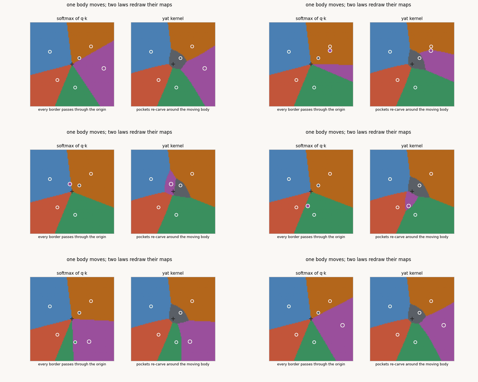

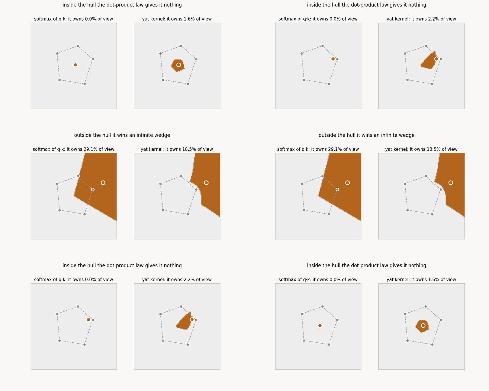
Two territory maps side by side while one body orbits: the softmax map's borders swing like spokes through the origin while the yat kernel map's pockets travel with the body — One body orbits; both maps recomputed from their formulas at every frame. Left: every border stays a line through the origin, so the moving body only re-aims wedges, and while it passes inside the others’ hull its color vanishes from the map entirely. Right: the body’s pocket travels with it. The toy scalars are the explainer’s: b at its log 2 initialization, softening below the body spacing.

The hull theorem gets its own animation, because its signature is a discontinuity you can watch for. The orange body walks a straight line from the center of the ring to well outside and back; each frame recomputes its territory share under both laws:

An orange body crossing a dashed convex hull: its softmax territory reads exactly zero percent inside, then an infinite wedge snaps into existence at the crossing, while its kernel pocket varies smoothly the whole way — The disenfranchisement theorem, watched. Inside the dashed hull the dot-product law’s counter reads exactly 0.0 percent, frame after frame, because the interior body’s score is a convex combination of the others’ and an average never beats its own maximum. At the crossing a wedge snaps into existence. The kernel’s share never touches zero: a well keeps the ground it stands on.

One ray, both readings

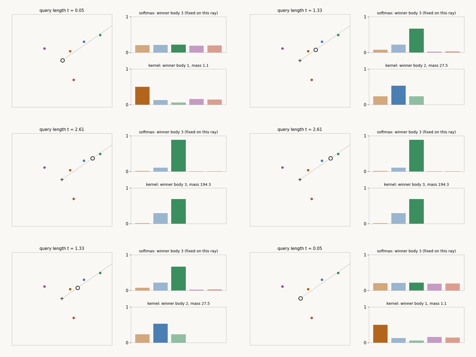
The scaling story is a one-dimensional process, so it animates as one: a query rides a ray out of the origin, and both weight rows are recomputed from the two formulas at every position:

A query dot traveling out along a dashed ray while two bar charts update: the softmax bars sharpen onto one fixed winner while the kernel bars hand the peak from body to body and a mass counter swells and dies — The same slider, two meanings. The softmax row keeps one winner for the entire ride and only concentrates onto it: the query’s length is an inverse temperature. The kernel row hands the peak from body to body as the query passes them, and its raw mass swells near a body and sags in the void: the length is an address.

The scale test on the trained model

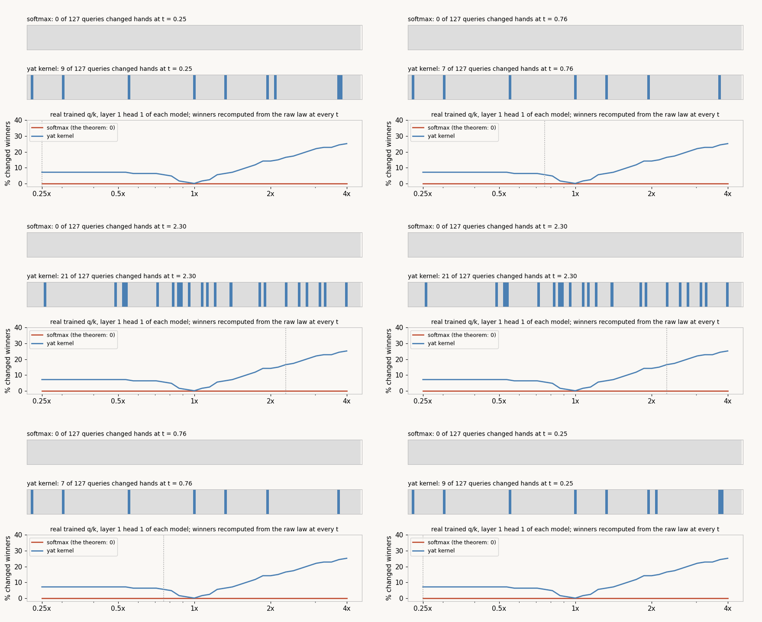
The explainer’s strongest claim, that no rescaling of any query can change a softmax winner, is checked on the real trained vectors by brute replay. For each row, at each scale $t$ , the score is rebuilt from the raw law; for the kernel that means reassembling the distance from the same dot products, with the head’s own learned scalars:

if model == "softmax":
    def score(t):
        return t * dots                    # argmax unaffected by /sqrt(dh)
else:
    b, eps = b_l[l][h], e_l[l][h]
    def score(t):
        d2 = (t * t) * qq[:, None] + kk2[None, :] - 2 * t * dots
        return (t * dots + b) ** 2 / (np.maximum(d2, 0.0) + eps)

queries scaled by	yat kernel	no Q/K tier
0.5x	12.1%	19.0%
2x	15.1%	16.7%
4x	23.3%	24.2%

The zeros are exact: 0 of 15,240 winner comparisons across all layers, heads, rows, and scales. The animation sweeps the same computation continuously on one head of each model:

Two strips of query columns and a curve: as the scale sweeps from a quarter to four, the softmax strip never lights and its curve sits on zero, while the kernel strip lights up progressively and its curve rises to about 25 percent — The real trained q/k of one head per model, every row’s winner recomputed at every scale. A column lights when its winner differs from the winner at t = 1. The softmax strip stays dark at every t, the theorem holding on a trained network to the digit; the kernel re-elects up to a quarter of its rows across the sixteen-fold sweep.

The census, through training

Ownership on the real window comes straight off the checkpointed maps: the winner of row $i$ is its argmax, and occupancy is how many distinct keys ever win:

win = attn.argmax(axis=-1).astype(np.int16)           # (L,H,T)
occ = len(set(win[l, h][first:].tolist())) / T        # distinct winners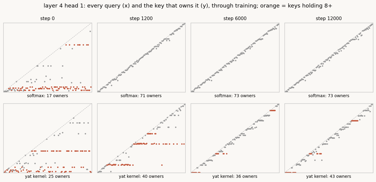

A two-by-four grid of ownership scatters, softmax over yat kernel, at training steps 0, 1200, 6000 and 12000: noise organizing into a diagonal ridge, with orange horizontal runs of annexed queries in the kernel row — One layer and head at the four telemetry checkpoints, both models: ownership organizing out of noise. Four snapshots are four facts, so this is a grid. The kernel row keeps its orange annexation runs, one key owning a stretch of queries, and ends with fewer distinct owners than the softmax head above it.

Averaged over all 24 heads, the softmax model’s occupancy climbs from 27 to 72 distinct winners out of 128 through training; the kernel’s from 31 to 54. Held against the entropy telemetry (0.49 versus 0.72 on this window), that is the inversion the explainer dwells on: the sharper-rowed model crowns more distinct winners, and row concentration and map concentration come apart as measurements.

The hull, by linear program

Whether a key sits inside the convex hull of its 127 siblings is a feasibility question, so it goes to a linear program: does a convex combination of the others reproduce this key exactly?

from scipy.optimize import linprog
others = np.delete(K, j, axis=0)                   # (T-1, dh)
A_eq = np.vstack([others.T, np.ones(T - 1)])
b_eq = np.concatenate([K[j], [1.0]])
r = linprog(np.zeros(T - 1), A_eq=A_eq, b_eq=b_eq,
            bounds=(0, None), method="highs")
inside = (r.status == 0)

Result: 0 interior keys of 3,072 in the softmax model, 0 of 3,072 in the kernel model. In 48 dimensions a generic cloud of 128 points is all hull, so the plane’s absolute disenfranchisement becomes, in the real network, the statistical statement the census already measured.

The far sky, on its schedule

The last animation is the explainer’s limit made visible, with its counter computed at every frame: the kernel’s owner map as the view zooms from radius 2 to 120, against the softmax map that provably cannot depend on the zoom at all. The antipodal-agreement statistic, the fraction of directions whose owner matches their opposite’s, climbs from 0 to 100 percent on the schedule the $1/t$ correction sets:

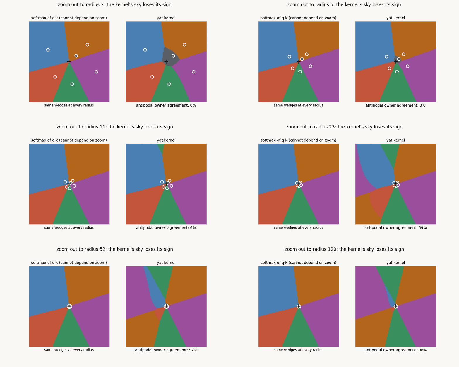
Two owner maps while the view zooms out: the softmax wedges are identical at every radius, while the yat kernel's pockets dissolve into wedges and an antipodal agreement counter climbs from zero to one hundred percent — Zooming out, both maps recomputed per frame. The softmax map is the same picture at every radius, which is the scale theorem wearing its other hat. The kernel’s pockets dissolve into wedges, and the counter shows the sign leaving: near the bodies antipodal directions have different owners, far away they agree, crossing 90 percent around radius 45 on these six bodies.

Every number is from seed-0 runs of scripts/yat_attention.py on Kaggle with TELEMETRY=1 GEOMETRY=1 (bundles kgl_blog-attngeom-qk, kgl_blog-attngeom-goat), analyzed locally by scripts/export_attention_geometry_viz.py; the toy animations compute the two laws’ formulas directly, with the explainer’s panel scalars. Quality numbers for these architectures, with seeds, live in the kernel-attention companion.

Cite as

Bouhsine, T. (2026, July 19). Measuring Attention's Geometry in JAX/Flax NNX. Records of the !mmortal Data Scientist. https://tahabouhsine.com/blog/the-geometry-of-attention-jax-flax-nnx/

BibTeX

@misc{bouhsine2026thegeometryofattentionjaxflaxnnx,
  author       = {Bouhsine, Taha},
  title        = {Measuring Attention's Geometry in JAX/Flax NNX},
  year         = {2026},
  month        = {jul},
  howpublished = {\url{https://tahabouhsine.com/blog/the-geometry-of-attention-jax-flax-nnx/}},
  note         = {Blog post, Records of the !mmortal Data Scientist}
}

References

Bouhsine, T. (2026). A Universal Reproducing Kernel Hilbert Space from Polynomial Alignment and IMQ Distance. arXiv:2605.03262

Exporting the geometry#

Two laws, two maps#

One ray, both readings#

The scale test on the trained model#

The census, through training#

The hull, by linear program#

The far sky, on its schedule#