Convolutional Autoencoder

Squeeze an image through a tiny latent bottleneck, then rebuild it — the simplest way to learn what a network chooses to keep.

Prerequisites

This guide builds on Simple CNN for the encoder and Simple Training Loop for the optimization pattern.

What you'll learn

• Build an encoder → bottleneck → decoder in Flax NNX by reusing shared ConvEncoder and ConvDecoder
• Use nnx.ConvTranspose to learn upsampling instead of fixed interpolation
• Train with a per-pixel sigmoid binary cross-entropy reconstruction loss
• Turn the same model into a denoising autoencoder by corrupting the input while keeping a clean target
• Track tensor shapes through the 28 → 7 → 28 bottleneck without flatten bugs

Example Code

Full runnable script: examples/generative/autoencoder.py

Why autoencoders?

An autoencoder learns to copy its input to its output — but through a narrow bottleneck that is far smaller than the input. Because the code $z$ cannot hold all 784 pixels of a 28×28 image, the network is forced to keep only the structure that matters for reconstruction and throw away noise. That pressure is what makes the latent code a useful, compressed representation.

Formally, we split the model into an encoder $f_\theta$ and a decoder $g_\phi$:

$$z = f_\theta(x) \in \mathbb{R}^d, \qquad \hat{x} = g_\phi(z), \qquad d \ll 784.$$

We train both halves jointly to minimize a reconstruction loss between the original $x$ and the reconstruction $\hat{x}$. For images with pixel values in $[0, 1]$, the decoder emits logits and we use per-pixel sigmoid binary cross-entropy, summed over pixels and averaged over the batch:

$$\mathcal{L}(x) = -\sum_{i} \Big[\, x_i \log \sigma(\ell_i) + (1 - x_i)\log\big(1 - \sigma(\ell_i)\big)\Big], \qquad \hat{x}_i = \sigma(\ell_i),$$

where $\ell_i$ is the decoder's output logit for pixel $i$ and $\sigma$ is the sigmoid. BCE is the natural choice when targets live in $[0, 1]$: it treats each pixel as a Bernoulli probability.

Why ConvTranspose upsamples

The encoder uses two stride-2 convolutions that halve the spatial size twice: $28 \to 14 \to 7$. To reconstruct, the decoder must go the other way, $7 \to 14 \to 28$. A transposed convolution (nnx.ConvTranspose) with stride 2 does exactly this: it spreads each input cell across a larger output window and learns the upsampling kernel, rather than relying on a fixed rule like nearest-neighbor or bilinear interpolation. Stacking two of them mirrors the encoder and returns to full resolution.

Building the model

We reuse the shared ConvEncoder (two stride-2 conv blocks) and ConvDecoder (a linear projection plus two nnx.ConvTranspose blocks), and add a nnx.Linear bottleneck in between.

import jax
import jax.numpy as jnp
from flax import nnx
import optax

from shared.models import ConvEncoder, ConvDecoder
from shared.training_utils import bce_loss


class ConvAutoencoder(nnx.Module):
    """Encoder -> Linear bottleneck -> Decoder."""

    def __init__(self, latent_dim: int = 32, base: int = 16,
                 in_channels: int = 1, *, rngs: nnx.Rngs):
        self.enc_hw = 7                      # 28 -> 14 -> 7 after two stride-2 convs
        self.enc_channels = base * 2         # ConvEncoder doubles `base`
        self.encoder = ConvEncoder(in_channels, base, rngs=rngs)
        # Bottleneck: squeeze the (7*7*base*2) feature map into `latent_dim`.
        self.bottleneck = nnx.Linear(
            self.enc_channels * self.enc_hw * self.enc_hw, latent_dim, rngs=rngs
        )
        # Decoder mirrors the encoder and returns LOGITS (no final activation).
        self.decoder = ConvDecoder(latent_dim, base, in_channels,
                                   start_hw=self.enc_hw, rngs=rngs)

    def encode(self, x):
        h = self.encoder(x)                  # (B, 7, 7, base*2)
        h = h.reshape(h.shape[0], -1)        # (B, 7*7*base*2)
        return self.bottleneck(h)            # (B, latent_dim)

    def __call__(self, x, train: bool = False):
        z = self.encode(x)                   # bottleneck code
        return self.decoder(z)               # (B, 28, 28, in_ch) logits

The shapes flow like this:

x            (B, 28, 28, 1)
ConvEncoder  (B,  7,  7, 32)   # two stride-2 convs, base=16 -> 32 channels
flatten      (B, 1568)
bottleneck   (B, 32)           # the compressed code z
ConvDecoder  (B, 28, 28, 1)    # two ConvTranspose steps: 7 -> 14 -> 28 (logits)

Instantiate it with an explicit nnx.Rngs and pair it with an optimizer:

model = ConvAutoencoder(latent_dim=32, rngs=nnx.Rngs(0))
optimizer = nnx.Optimizer(model, optax.adam(1e-3), wrt=nnx.Param)

The training step

The train step is the standard NNX pattern: a loss_fn closed over the model, nnx.value_and_grad, then optimizer.update. The batch carries a (possibly corrupted) input x and a clean target; for a plain autoencoder they are the same array.

@nnx.jit
def train_step(model, optimizer, batch):
    def loss_fn(model):
        logits = model(batch['x'], train=True)      # (B, 28, 28, 1)
        loss = bce_loss(logits, batch['target'])    # sigmoid-BCE per pixel
        return loss, logits

    (loss, logits), grads = nnx.value_and_grad(loss_fn, has_aux=True)(model)
    optimizer.update(model, grads)
    return loss, logits

Denoising variant

A denoising autoencoder keeps the exact same model and loss, but corrupts the input with Gaussian noise while asking the decoder to reproduce the clean image:

$$\tilde{x} = \operatorname{clip}(x + \epsilon,\ 0,\ 1), \qquad \epsilon \sim \mathcal{N}(0, \sigma^2 I), \qquad \min_{\theta, \phi}\ \mathcal{L}\big(x,\ g_\phi(f_\theta(\tilde{x}))\big).$$

Because the target is clean but the input is not, the network can no longer just memorize an identity map — it has to model how pixels relate so it can fill in what the noise destroyed.

def add_gaussian_noise(x, key, std: float):
    """Corrupt inputs with Gaussian noise, then clip back to [0, 1]."""
    noisy = x + std * jax.random.normal(key, x.shape)
    return jnp.clip(noisy, 0.0, 1.0)


def make_batch(images, idx, *, denoising: bool, noise_std: float, key):
    clean = images[idx]
    x = add_gaussian_noise(clean, key, noise_std) if denoising else clean
    return {'x': x, 'target': clean}          # input vs. clean target

Flip denoising on (the script reads a DENOISE=1 env var) and everything else — model, loss, optimizer — stays identical.

Results / What to Expect

The script defaults to tiny, offline synthetic binarized images (no downloads), so it runs on CPU in seconds. The BCE loss is summed over all 784 pixels, so it lives in the hundreds. Note the synthetic data is pure random noise with no structure to compress, so it sits near its entropy floor and the loss creeps down only slowly — the point of the synthetic default is that it runs offline and the loss decreases, not that it reaches zero. On real MNIST (SYNTHETIC=0) the digits are far more compressible and the loss falls much faster.

$ python generative/autoencoder.py
Convolutional autoencoder on synthetic data
  epochs=4 batch=64 latent_dim=32 noise_std=0
  dataset: (512, 28, 28, 1)  (clean targets in [0, 1])
  epoch  1/4 | steps    8 | BCE   543.54
  epoch  2/4 | steps   16 | BCE   543.21
  epoch  3/4 | steps   24 | BCE   542.85
  epoch  4/4 | steps   32 | BCE   542.26
Done. The decoder's nnx.ConvTranspose layers upsample 7->14->28.

If you want to watch the loss drop sharply, run more steps on a single fixed batch (as the verification below does): on 30 steps of one batch it falls from ~544 to ~468.

On real MNIST (SYNTHETIC=0, LATENT=64, 60 epochs) the reconstructions come back through the bottleneck as recognizable digits — the whole point of the autoencoder:

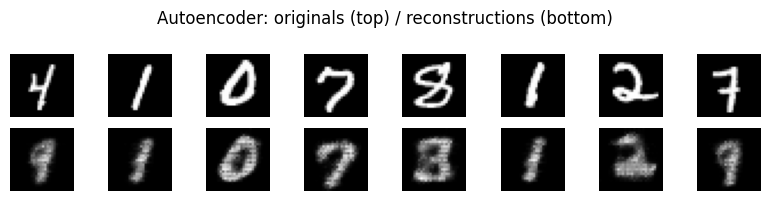
Top: real inputs. Bottom: each image squeezed through a 64-dim bottleneck and rebuilt by the nnx.ConvTranspose decoder. Blurrier than the input (the bottleneck discards detail) but clearly the same digit — the network learned to compress and reconstruct.

Run the denoising variant with DENOISE=1 python generative/autoencoder.py, or point it at MNIST with SYNTHETIC=0.

Common Pitfalls

❌ Applying a sigmoid inside the decoder, then also using sigmoid-BCE. ✅ Have the decoder return raw logits and let bce_loss (which wraps optax.sigmoid_binary_cross_entropy) apply the sigmoid once — double-sigmoid squashes gradients.

❌ Hardcoding the flatten size, e.g. h.reshape(B, 1568), which breaks if base or the input size changes. ✅ Use h.reshape(h.shape[0], -1) so the bottleneck input dimension is derived from the tensor.

❌ Reconstructing the noisy input in the denoising variant (target = noisy). ✅ Corrupt only batch['x']; keep batch['target'] the clean image, or the model just learns to copy noise.

❌ Making the bottleneck as wide as the input (e.g. latent_dim=784). ✅ Keep $d \ll 784$ (32 works well here) so the network is forced to compress instead of learning an identity map.

❌ Putting the encoder/decoder submodules in a plain Python list. ✅ On Flax 0.12 wrap any list of submodules in nnx.List([...]) (the shared ConvEncoder/ConvDecoder already store their layers correctly).

Next steps

• Variational Autoencoders (VAE) — put a probability distribution over the latent code and sample new digits.
• Generative Adversarial Networks (GAN) — generate sharp images with an adversarial game instead of a reconstruction loss.

Complete Example

examples/generative/autoencoder.py — a runnable convolutional autoencoder with a denoising flag, synthetic-by-default data, and an MNIST switch.

References

• Bengio, Courville & Vincent, Representation Learning: A Review and New Perspectives (2013) — autoencoders as representation learners.
• Dumoulin & Visin, A Guide to Convolution Arithmetic for Deep Learning (2016) — how transposed convolutions upsample.
• Kingma & Welling, Auto-Encoding Variational Bayes (2013) — the probabilistic extension covered in the VAE guide.