Normalizing Flows (RealNVP)

Learn an exact, invertible density: turn two crescent moons into a Gaussian, then run the map backwards to sample brand-new points.

Prerequisites

• Variational Autoencoder (VAE) — the encoder/decoder generative baseline this guide contrasts with.
• Simple Training Loop — the nnx.value_and_grad + optimizer.update pattern reused here.

What you'll learn

• The change-of-variables formula and why an invertible network gives you exact log-likelihood (no ELBO, no adversary).
• How an affine coupling layer stays invertible while its Jacobian log-determinant collapses to a simple sum(s).
• Why stacking layers with alternating masks lets every dimension get transformed.
• Training a flow by maximum likelihood — minimizing the mean negative log-density directly.
• Using one network for two directions: forward (data → base) to score, inverse (base → data) to sample.

Example Code

The complete, runnable script for this guide lives at examples/generative/normalizing_flows.py.

Why an invertible model?

A VAE only ever gives you a lower bound on the likelihood, and a GAN gives you no likelihood at all. A normalizing flow takes a different bargain: build the generator out of invertible transformations so you can compute the data density exactly.

The idea is to warp a simple base distribution — here a standard normal $p_Z = \mathcal{N}(0, I)$ — into the complicated data distribution through a learnable bijection $f$. If $z = f(x)$ is invertible and differentiable, the change-of-variables formula gives the density of $x$ exactly:

$$\log p_X(x) = \log p_Z\big(f(x)\big) + \log\left|\det \frac{\partial f(x)}{\partial x}\right|$$

Two directions fall out of one model:

• Score / train — push data through the forward map $x \to z$, evaluate the base density and the log-determinant, and maximize $\log p_X(x)$.
• Sample — draw $z \sim \mathcal{N}(0, I)$ and run the map backwards, $x = f^{-1}(z)$.

The catch is the $\log|\det|$ term: for a general network the Jacobian determinant costs $O(d^3)$. RealNVP solves this with a layer whose Jacobian is triangular, so the determinant is just the product of its diagonal.

Affine coupling layers

RealNVP splits the input into two halves. One half passes through untouched and conditions an affine transform (scale and shift) applied to the other half. We select the halves with a binary mask $m \in \{0, 1\}^d$:

$$\begin{aligned} z &= m \odot x \;+\; (1 - m) \odot \big(x \odot e^{s(m \odot x)} + t(m \odot x)\big) \\ \log\left|\det \frac{\partial z}{\partial x}\right| &= \sum_j (1 - m_j)\, s_j \end{aligned}$$

Because the kept half is copied verbatim and the transformed half depends on it only through $s$ and $t$, the Jacobian is triangular — its log-determinant is simply the sum of the scales $s$. The network predicting $s$ and $t$ can be arbitrarily complex; invertibility never depends on it.

Inverting is closed-form. Given $z$, the kept half already equals $x$'s kept half, so we recompute the same $s$ and $t$ and undo the affine map:

$$x = m \odot z \;+\; (1 - m) \odot (z - t) \odot e^{-s}$$

A single layer leaves half the dimensions unchanged, so we stack layers and alternate the mask parity. After two layers every dimension has been both a conditioner and a transform target.

from flax import nnx
import jax.numpy as jnp
from shared.models import MLP

class AffineCoupling(nnx.Module):
    def __init__(self, dim: int, hidden: int, parity: int, *, rngs: nnx.Rngs):
        self.dim = dim
        self.parity = parity
        # Conditioner: (kept dims) -> concat[s_raw, t], each of size `dim`.
        self.net = MLP(dim, hidden, 2 * dim, n_layers=2, rngs=rngs, activation="gelu")

    def _mask(self):
        # 1.0 where a dim is kept (conditions), 0.0 where it is transformed.
        return (jnp.arange(self.dim) % 2 == self.parity).astype(jnp.float32)

    def _s_t(self, u, mask):
        s_raw, t = jnp.split(self.net(u * mask), 2, axis=-1)
        s = jnp.tanh(s_raw) * (1.0 - mask)   # bounded scale, transformed dims only
        t = t * (1.0 - mask)                 # shift, transformed dims only
        return s, t

    def forward(self, x):
        mask = self._mask()
        s, t = self._s_t(x, mask)
        z = x * mask + (1.0 - mask) * (x * jnp.exp(s) + t)
        logdet = jnp.sum(s, axis=-1)
        return z, logdet

    def inverse(self, z):
        mask = self._mask()
        s, t = self._s_t(z, mask)  # kept dims == x's kept dims, so s,t match
        x = z * mask + (1.0 - mask) * (z - t) * jnp.exp(-s)
        return x

We squash the raw scale with tanh so $e^{s}$ stays in a stable range — a common RealNVP trick that keeps early training from exploding.

Stacking into a flow

The RealNVP module composes the coupling layers. forward accumulates the total log-determinant; inverse replays the layers in reverse. log_prob glues them to the standard-normal base, and sample runs the flow backwards from base noise.

import jax
import jax.numpy as jnp

class RealNVP(nnx.Module):
    def __init__(self, dim=2, hidden=64, n_layers=6, *, rngs: nnx.Rngs):
        self.dim = dim
        # A plain list of submodules MUST be wrapped in nnx.List on Flax 0.12.
        self.layers = nnx.List([
            AffineCoupling(dim, hidden, parity=i % 2, rngs=rngs)
            for i in range(n_layers)
        ])

    def forward(self, x):
        logdet = jnp.zeros(x.shape[0])
        z = x
        for layer in self.layers:
            z, ld = layer.forward(z)
            logdet = logdet + ld
        return z, logdet

    def inverse(self, z):
        x = z
        for i in range(len(self.layers) - 1, -1, -1):
            x = self.layers[i].inverse(x)
        return x

    def log_prob(self, x):
        z, logdet = self.forward(x)
        # log N(z; 0, I) = -0.5||z||^2 - 0.5 d log(2*pi)
        logpz = -0.5 * jnp.sum(z ** 2, axis=-1) - 0.5 * self.dim * jnp.log(2.0 * jnp.pi)
        return logpz + logdet

    def sample(self, n: int, seed: int = 0):
        z = jax.random.normal(jax.random.key(seed), (n, self.dim))
        return self.inverse(z)

nnx.List is required

A raw Python list of submodules is invisible to Flax 0.12's pytree machinery — their parameters won't register and training crashes. Always wrap submodule lists in nnx.List([...]) (and dicts in nnx.Dict({...})).

The loss and train step

Training a flow is refreshingly direct: minimize the mean negative log-likelihood. There's no lower bound and no discriminator — the model reports its own exact density.

def nll_loss(model, x):
    return -model.log_prob(x).mean()

The train step is the standard NNX pattern — nnx.value_and_grad with has_aux=True, then optimizer.update(model, grads):

@nnx.jit
def train_step(model, optimizer, batch):
    def loss_fn(model):
        nll = nll_loss(model, batch)
        return nll, nll   # aux = nll for logging

    (loss, aux), grads = nnx.value_and_grad(loss_fn, has_aux=True)(model)
    optimizer.update(model, grads)
    return loss, aux

Wire it up with a single RNG stream and Adam:

import optax

rngs = nnx.Rngs(0)
model = RealNVP(dim=2, hidden=64, n_layers=6, rngs=rngs)
optimizer = nnx.Optimizer(model, optax.adam(1e-3), wrt=nnx.Param)

The data: two moons, no sklearn

We generate the classic two-moons set ourselves from two noisy half circles and standardize it so the $\mathcal{N}(0, I)$ base is a good target — fully offline, no downloads.

def make_two_moons(n=1024, noise=0.1, seed=0):
    key = jax.random.key(seed)
    k1, k2, k3 = jax.random.split(key, 3)
    n_out, n_in = n // 2, n - n // 2

    t_out = jnp.pi * jax.random.uniform(k1, (n_out,))
    outer = jnp.stack([jnp.cos(t_out), jnp.sin(t_out)], axis=1)

    t_in = jnp.pi * jax.random.uniform(k2, (n_in,))
    inner = jnp.stack([1.0 - jnp.cos(t_in), 1.0 - jnp.sin(t_in) - 0.5], axis=1)

    x = jnp.concatenate([outer, inner], axis=0)
    x = x + noise * jax.random.normal(k3, x.shape)
    return (x - x.mean(0)) / (x.std(0) + 1e-6)   # standardize per dim

Results / What to expect

The script defaults to tiny synthetic data so it runs offline on CPU in seconds. The mean negative log-likelihood falls steadily as the flow warps the moons onto the Gaussian:

$ python generative/normalizing_flows.py
epoch 1/8  nll 2.9005
epoch 2/8  nll 2.6915
epoch 3/8  nll 2.6044
epoch 4/8  nll 2.5378
epoch 5/8  nll 2.4859
epoch 6/8  nll 2.4423
epoch 7/8  nll 2.4069
epoch 8/8  nll 2.3750
samples: (256, 2)  latent: (256, 2)

At the end of training the script draws fresh samples with model.sample and plots them next to the real data:

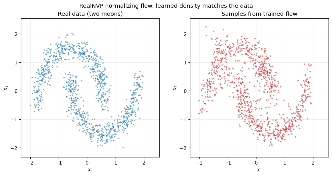
Left: the real two-moons data. Right: points obtained by drawing $z \sim \mathcal{N}(0, I)$ and pushing them through inverse. The samples reproduce the same two crescents — visual proof that the flow learned the true density, not just a low number.

Two invariants make this model trustworthy, and the example verifies both:

• Exact invertibility — inverse(forward(x)) reconstructs x to ~1e-6 (float32 round-off), confirming the affine coupling is a true bijection.
• Faithful sampling — model.sample(n, seed) returns (n, 2) points that, once training converges, trace out the two crescents. Because the flow is exact, those samples come straight from z ~ N(0, I) pushed through inverse.

Tune EPOCHS, BATCH, and SYNTHETIC (dataset size) via environment variables to trade runtime for a sharper fit.

Common Pitfalls

• ❌ Storing submodules in a plain Python list, so their params never register. ✅ Wrap them in nnx.List([...]) (and dicts in nnx.Dict({...})) on Flax 0.12.

• ❌ Letting the scale $s$ run unbounded — exp(s) overflows to inf/NaN early. ✅ Squash it: s = jnp.tanh(s_raw), keeping $e^{s}$ in a stable band.

• ❌ Forgetting the $\log|\det|$ term and training on -log p_z(f(x)) alone. ✅ Return logpz + logdet from log_prob; without the Jacobian term the model cheaply collapses all mass to one point.

• ❌ Running the same layer order for inverse as forward. ✅ Apply layers in reverse during inverse — a flow is $f_L \circ \dots \circ f_1$, so its inverse is $f_1^{-1} \circ \dots \circ f_L^{-1}$.

• ❌ Feeding raw, unscaled two-moons into a $\mathcal{N}(0, I)$ base. ✅ Standardize the data (zero mean, unit variance) so the base is a reachable target.

Next steps

• Diffusion Models (DDPM) — another exact-ish likelihood generator that trades one invertible map for many denoising steps.
• Generative Adversarial Networks (GAN) — the likelihood-free alternative that learns the density implicitly.

Complete Example

The full, verified script is at examples/generative/normalizing_flows.py — a CPU-friendly RealNVP with synthetic two-moons defaults, exact-likelihood training loop, invertibility check, and a sample() generator.

References

• Dinh, Sohl-Dickstein & Bengio, Density Estimation using Real NVP (2016). arXiv:1605.08803
• Dinh, Krueger & Bengio, NICE: Non-linear Independent Components Estimation (2014). arXiv:1410.8516
• Rezende & Mohamed, Variational Inference with Normalizing Flows (2015). arXiv:1505.05770
• Papamakarios et al., Normalizing Flows for Probabilistic Modeling and Inference (2019). arXiv:1912.02762