 JAX Pathways
Phase 03 / State, randomness & control flow
Compiled loops with lax.scan
Revision v0.7.0 · Updated since your last visit. Review the changes; your progress is saved.
Lesson · about 65 minutes · CPU practice
Replace a fixed-length Python loop with scan and compare final states.
Phase study guide: preparation, milestones and project evidence
Before you start
Before this: Pytrees and structured parameters
Hardware: CPU
Setup help: Python, notebook, or Cloud TPU VM
Use the tested CPU packages (the recorded environment uses Python 3.14.3). Other Python versions and accelerator environments require separate checks. The optional Cloud TPU specialization explains the target-specific execution boundaries. Logical CPU devices practice partitioning; they do not simulate TPU performance.
Download the repository ZIP or use your existing checkout. Extract it and open a terminal in the folder containing requirements-cpu.txt. The beginner ZIP is separate; these lessons use the full repository folder.
python3 -m venv .venv
source .venv/bin/activate
python -m pip install -r requirements-cpu.txtpy -3 -m venv .venv
.\.venv\Scripts\python.exe -m pip install -r requirements-cpu.txtAfter activation, run the complete worked example from that same folder:
python phases/03-state/03-compiled-loops-with-lax-scan/code/main.py.\.venv\Scripts\python.exe phases/03-state/03-compiled-loops-with-lax-scan/code/main.pyFor an incremental build, create main.py in your own practice folder, append each build block in order, and run python main.py with this environment active. Keep that file separate from the downloaded reference solution.
Download this lesson’s notebook. Open it with a Python kernel using the course environment. Run cells from the top after restarting the kernel; experiments depend on earlier definitions.
For local Jupyter, first install the course requirements using the Local Python steps, then use your environment’s Python to start Jupyter:
python -m pip install jupyterlab
python -m jupyter lab.\.venv\Scripts\python.exe -m pip install jupyterlab
.\.venv\Scripts\python.exe -m jupyter labSelect the downloaded state-03.ipynb file in JupyterLab. The notebook contains reference solutions; make your prediction and attempt each practice task before opening them. Restart the kernel before changing logical device setup.
The worked reference for this lesson is CPU-validated. Some references explicitly configure logical CPU devices; setting JAX_PLATFORMS does not adapt them to a TPU. Follow the execution matrix and reviewed multi-host example before attempting a target run.
For accelerator preparation, study TPU setup, observed runtime receipts, checkpointed jobs and precision and retained traces. These target paths remain unqualified on physical TPU hardware until an actual receipt is recorded. Cloud provisioning is optional for CPU learning.
Check: History: ; Final: .
Revisit the guided CPU setup · Open 19: TPU Setup. Package instructions are CPU instructions; Windows and accelerator environments need their own validation.
What you will be able to do
- Separate carry from recorded outputs
- Keep the carry contract invariant
- Differentiate the recurrence by hand
- Compile the repeated transition without a timing promise
The problem
Suppose a simulator keeps part of its current value and adds a new input at each step. Let’s write out four steps so we know what should happen. Then we’ll express the same loop with scan, compare it with Python, and see how changing the retained fraction affects the final value.
The idea
A scan separates the state carried between steps from the outputs collected at each step. This is useful whenever the same rule repeats over time while the state keeps a fixed structure, shape and dtype.
- Initial state
carry₀, inputs[0]Start with an explicit state tree.
- Body
carry₁, output₀ = body(carry₀, input₀)Return the next state and this step’s output.
- Repeat
carryₜ → body → carryₜ₊₁scan collects outputs and returns the final carry.
Every carry leaf keeps the same shape and dtype through the loop. Outputs are stacked along the scan axis; the carry is the state that connects steps.
Conceptual illustration. Verify the computation in the lesson’s Python experiments.
Unroll three steps before compiling the loop
For a separate hand-worked recurrence, start with carry and inputs . Let each step add its input to the carry and emit the new carry. The successive carries are ; the final carry is , while the stacked outputs are .
Those two returned objects answer different questions. Keeping only the final carry discards the intermediate outputs. Keeping outputs does not mean the carry itself grows on each iteration. A fixed carry contract is what makes the repeated computation structured.
Trace one horizontal state edge and one downward output edge in the diagram. When adapting a Python loop, write down which variables belong on each edge before translating the loop to lax.scan.
Carry moves through time; outputs are collected
Predict: What changes if the step emits the old carry instead of the new carry?
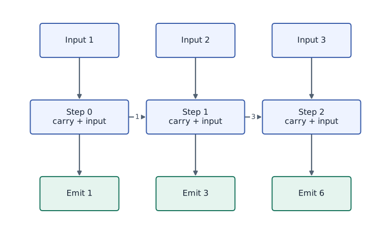
An additive scan starts with carry and inputs . Horizontal arrows pass updated carry; downward arrows collect emitted values. Final carry and outputs are different return values. Arrow lengths do not represent runtime.
Separate carry from recorded outputs
Each scan step receives (carry,input) and returns (next_carry,output). Carry is what the next step needs. Output is what you want stacked into a history. They can have different meanings even when this demonstration returns the new state in both positions.
For decay , initial state and four inputs of , the states are ,,,. There are four recorded outputs; the initial state is not automatically part of history. Decide whether a plot should include that initial point before labeling the time axis.
(state_t, input_t) → transition → (state_(t+1), recorded_t)
state: 0 → 1 → 1.5 → 1.75 → 1.875
Keep the carry contract invariant
Carry values change, but their pytree structure, shapes and dtypes must remain compatible across steps. Growing a Python list or concatenating a larger array into the carry changes that contract. Allocate a fixed-size state or use the separately stacked outputs instead.
This constraint is a representation decision, not an arbitrary restriction on simulation. A fixed-dimensional physical state naturally meets it. If a system has variable numbers of entities, consider padding and masks with an explicit maximum capacity.
Differentiate the recurrence by hand
With four unit inputs and initial zero, the final value is . Its derivative is , giving at . The derivative also obeys a recurrence: , starting from .
Autodiff through scan differentiates the represented state transition. It does not make an unstable or inaccurate numerical model valid. Verify a small analytic case first, then a changed input sequence, before trusting a longer simulation.
Compile the repeated transition without a timing promise
A Python loop inside jit can be unrolled while tracing; scan expresses a repeated operation compactly. That can reduce compilation work for long loops, but it is not a universal promise that scan is faster for every workload.
Before benchmarking, compare numerical results on the same inputs and synchronize execution. Keep step count and precision explicit. For this lesson we verify correctness and derivatives; hardware profiling belongs to a later course unit.
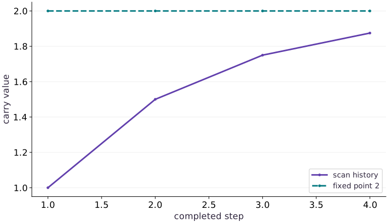
The carry approaches a fixed point
Predict before looking: Why does the increment between successive states shrink?
Read the figure
The solid line shows the carry after each completed scan step. It starts at step with value , then rises through , , and . The dashed horizontal line marks the fixed point .
The initial carry is not plotted. Each visible point is the value after applying the recurrence once more, so the first point already includes one update.
Connect it to the computation
The update is . Subtracting it from the fixed point gives : each step halves the remaining gap. This explains both the upward movement and its slowing pace.
The shrinking gaps are , , , and . scan carries the evolving value forward while collecting this history. One more step would produce ; it would not add another full unit or restart from the initial carry.
Open full-size figureDownload data and provenance
The notebook contains the data experiment, plotting code, and recorded figure output. Rerun it to test your changes.
Where to put & run this code: Work in phases/03-state/03-compiled-loops-with-lax-scan/code/main.py (or downloaded exercises/state-03.py / exercises/state-03.ipynb) and execute from the repository root with python3 phases/03-state/03-compiled-loops-with-lax-scan/code/main.py.
1 Prepare the inputs
Create main.py in your lesson workspace. Add this first block; use the environment from setup.
# Step 1 — Prepare the inputs: These explicit inputs define the case that the later checks will...
import jax
import jax.numpy as jnp
These explicit inputs define the case that the later checks will verify.
2 Build the computation
Append this block below the inputs in the same file.
# Step 2 — Build the computation: step returns the next scalar carry and one recorded scalar.
def step(carry, increment):
    next_value = 0.5 * carry + increment
    return next_value, next_value
increments = jnp.array([1., 1., 1., 1.])
Code building blocks in this step
jnp.array(values, dtype=...)— Constructs an immutable device-backed JAX array from Python/NumPy values.
step returns the next scalar carry and one recorded scalar. scan feeds that carry back into step and stacks the four recorded outputs.
3 Run and check the result
Append the checks, save main.py, and run python main.py from this folder using your course environment.
# Step 3 — Run and check the result: Compare the output to the expected result below before making the...
# Run compiled structured control flow via `jax.lax` (`(final, history)`).
final, history = jax.lax.scan(step, jnp.array(0.), increments)
print("History:", history)
print("Final:", float(final))
assert jnp.allclose(history, jnp.array([1.,1.5,1.75,1.875]))
assert jnp.allclose(final, history[-1])
Code building blocks in this step
jnp.array(values, dtype=...)— Constructs an immutable device-backed JAX array from Python/NumPy values.jnp.allclose(actual, expected, rtol=..., atol=...)— Checks that two arrays match elementwise within floating-point tolerance.jax.lax.scan(step_fn, init_carry, xs, length=...)— Compiles a sequential loop wherestep_fn(carry, x)returns(next_carry, y), returning(final_carry, stacked_ys).
Compare the output to the expected result below before making the exercise change.
View the cumulative build in main.py
These blocks append in order to the same file.
# Step 1 — Prepare the inputs: These explicit inputs define the case that the later checks will...
import jax
import jax.numpy as jnp

# Step 2 — Build the computation: step returns the next scalar carry and one recorded scalar.
def step(carry, increment):
    next_value = 0.5 * carry + increment
    return next_value, next_value
increments = jnp.array([1., 1., 1., 1.])

# Step 3 — Run and check the result: Compare the output to the expected result below before making the...
# Run compiled structured control flow via `jax.lax` (`(final, history)`).
final, history = jax.lax.scan(step, jnp.array(0.), increments)
print("History:", history)
print("Final:", float(final))
assert jnp.allclose(history, jnp.array([1.,1.5,1.75,1.875]))
assert jnp.allclose(final, history[-1])
Run the example
python3 phases/03-state/03-compiled-loops-with-lax-scan/code/main.pyAbout this command
This shortcut uses an activated macOS/Linux course environment in the repository folder. For Windows, use the explicit interpreter command in “Setup help” above. The script includes worked examples and reference solutions.
Inspect the complete assembled example
# Step 1 — Prepare the inputs: These explicit inputs define the case that the later checks will...
import jax
import jax.numpy as jnp
# Step 2 — Build the computation: step returns the next scalar carry and one recorded scalar.
def step(carry, increment):
    next_value = 0.5 * carry + increment
    return next_value, next_value
increments = jnp.array([1., 1., 1., 1.])
# Step 3 — Run and check the result: Compare the output to the expected result below before making the...
# Run compiled structured control flow via `jax.lax` (`(final, history)`).
final, history = jax.lax.scan(step, jnp.array(0.), increments)
print("History:", history)
print("Final:", float(final))
assert jnp.allclose(history, jnp.array([1.,1.5,1.75,1.875]))
assert jnp.allclose(final, history[-1])
Expected result: History: ; Final: .
Recorded reference execution
Reference output captured from executing the complete lesson script (code/main.py) and its assertions in the course CPU environment.
History: [1.    1.5   1.75  1.875]
Final: 1.875
History: [1.    1.5   1.75  1.875]
Final: 1.875
Expected carry-shape mismatch
PASS: state-03
Download execution record · The notebook includes executed cells and figure outputs. Compare your run with these values; timings depend on the machine.
Compare scan to the Python recurrence
# Experiment — Compare scan to the Python recurrence: The loop is an independent control-flow reference and the fixed...
inputs=jnp.array([1.,-1.,2.,0.])
state=0.
reference=[]
for inc in [1.,-1.,2.,0.]:
    state=0.5*state+inc
    reference.append(state)
# Run compiled structured control flow via `jax.lax` (`(last, observed)`).
last,observed=jax.lax.scan(step,jnp.array(0.),inputs)
assert jnp.allclose(observed,jnp.array([1.,-0.5,1.75,0.875]))
assert jnp.allclose(observed,jnp.array(reference))
assert jnp.allclose(last,state)
Expected: History ; final .
The loop is an independent control-flow reference and the fixed numbers verify time indexing.
Verify state and sensitivity together
# Experiment — Verify state and sensitivity together: The scalar objective is the final state.
# Define `terminal(d)` to carry state across steps with `jax.lax.scan`:
def terminal(d):
    return jax.lax.scan(lambda c,u:(d*c+u,d*c+u),jnp.array(0.),increments)[0]
# Differentiate the objective to obtain `(value, sensitivity)` via automatic differentiation.
value,sensitivity=jax.value_and_grad(terminal)(0.5)
assert jnp.allclose(value,1.875)
assert jnp.allclose(sensitivity,2.75)
assert jnp.allclose(jax.jit(terminal)(0.5),value)
Expected: Final state and sensitivity .
The scalar objective is the final state. Returning the whole history to ordinary grad would need a deliberate scalar reduction.
Make it yours
Where to put your code: Append your solution at the bottom of phases/03-state/03-compiled-loops-with-lax-scan/code/main.py (or inside the Make it yours cell of exercises/state-03.ipynb) and run python3 phases/03-state/03-compiled-loops-with-lax-scan/code/main.py to verify your prediction before opening the reference solution.
Make the decay an explicit scalar argument. Differentiate the final value with respect to decay and compare at with the analytic derivative .
Show a writing guide and starter scaffold
How to write this exercise code: step-by-step recipe & starter scaffold
1. Key functions & syntax to use:
jnp.array(values, dtype=...)— Constructs an immutable device-backed JAX array from Python/NumPy values.jnp.allclose(actual, expected, rtol=..., atol=...)— Checks that two arrays match elementwise within floating-point tolerance.jax.grad(loss_fn)(params, ...)— Transforms a scalar-output function into a function returning the gradient PyTree with the same structure asparams.jax.lax.scan(step_fn, init_carry, xs, length=...)— Compiles a sequential loop wherestep_fn(carry, x)returns(next_carry, y), returning(final_carry, stacked_ys).
2. Step-by-step implementation plan:
- Define
simulate(decay)to carry state across steps withjax.lax.scan:
# Exercise solution: Make the decay an explicit scalar argument.
# Define `simulate(decay)` to carry state across steps with `jax.lax.scan`:
def simulate(decay):
    def transition(carry, increment):
        value = ...  # TODO: compute value
        return ...  # TODO: return computed result
    return ...  # TODO: return computed result
assert jnp.allclose(jax.grad(simulate)(0.5), 2.75)  # TODO: complete assertion check
Reveal the reference solution
# Exercise solution: Make the decay an explicit scalar argument.
# Define `simulate(decay)` to carry state across steps with `jax.lax.scan`:
def simulate(decay):
    def transition(carry, increment):
        value = decay * carry + increment
        return value, value
    return jax.lax.scan(transition, jnp.array(0.), increments)[0]
assert jnp.allclose(jax.grad(simulate)(0.5), 2.75)
Record a different output
Practice
Carry the state, but record its squared value. Confirm that final carry still means state.
Show a writing guide and starter scaffold
How to write this practice solution: step-by-step recipe & starter scaffold
1. Key functions & syntax to use:
jnp.array(values, dtype=...)— Constructs an immutable device-backed JAX array from Python/NumPy values.jnp.allclose(actual, expected, rtol=..., atol=...)— Checks that two arrays match elementwise within floating-point tolerance.jax.lax.scan(step_fn, init_carry, xs, length=...)— Compiles a sequential loop wherestep_fn(carry, x)returns(next_carry, y), returning(final_carry, stacked_ys).
2. Step-by-step implementation plan:
- Run compiled structured control flow via
jax.lax((last, energy)).
# Record a different output (Practice): Carry and history need not have the same interpretation.
# Run compiled structured control flow via `jax.lax` (`(last, energy)`).
last,energy = jax.lax.scan(...)  # TODO: compute last,energy
assert jnp.allclose(last,1.875)  # TODO: complete assertion check
assert jnp.allclose(energy,jnp.array([1.,2.25,3.0625,3.515625]))  # TODO: complete assertion check
Show a hint
The second returned value is only the recorded output.
Reveal reference solution and reasoning
# Record a different output (Practice): Carry and history need not have the same interpretation.
# Run compiled structured control flow via `jax.lax` (`(last, energy)`).
last,energy=jax.lax.scan(lambda c,u:(0.5*c+u,(0.5*c+u)**2),jnp.array(0.),increments)
assert jnp.allclose(last,1.875)
assert jnp.allclose(energy,jnp.array([1.,2.25,3.0625,3.515625]))
Carry and history need not have the same interpretation. The state remains unsquared for the next transition.
Diagnose a growing carry
Challenge
Try appending each input to the carry with concatenate. Explain why scan rejects it and replace it with stacked output.
Show a writing guide and starter scaffold
How to write this practice solution: step-by-step recipe & starter scaffold
1. Key functions & syntax to use:
jnp.array(values, dtype=...)— Constructs an immutable device-backed JAX array from Python/NumPy values.jnp.zeros / jnp.ones(shape, dtype=...)— Allocates a tensor of the givenshapeinitialized with constants.jax.lax.scan(step_fn, init_carry, xs, length=...)— Compiles a sequential loop wherestep_fn(carry, x)returns(next_carry, y), returning(final_carry, stacked_ys).
2. Step-by-step implementation plan:
- Run the boundary check and catch the expected exception:
- Run compiled structured control flow via
jax.lax((_, saved)).
# Diagnose a growing carry (Challenge): The error identifies incompatible carry input/output types.
def growing(c,u):
    return ...  # TODO: return computed result
# Run the boundary check and catch the expected exception:
try:
    jax.lax.scan(growing,jnp.zeros((0,)),increments)
except TypeError:
    print("Expected carry-shape mismatch")
else:
    raise AssertionError("Expected scan type failure")
# Run compiled structured control flow via `jax.lax` (`(_, saved)`).
_,saved = jax.lax.scan(...)  # TODO: compute _,saved
assert jnp.array_equal(saved,increments)  # TODO: complete assertion check
Show a hint
The carry shape is part of the loop type.
Reveal reference solution and reasoning
# Diagnose a growing carry (Challenge): The error identifies incompatible carry input/output types.
def growing(c,u):
    return jnp.concatenate([c,u[None]]),u
# Run the boundary check and catch the expected exception:
try:
    jax.lax.scan(growing,jnp.zeros((0,)),increments)
except TypeError:
    print("Expected carry-shape mismatch")
else:
    raise AssertionError("Expected scan type failure")
# Run compiled structured control flow via `jax.lax` (`(_, saved)`).
_,saved=jax.lax.scan(lambda c,u:(c,u),jnp.array(0.),increments)
assert jnp.array_equal(saved,increments)
The error identifies incompatible carry input/output types. Store per-step values in scan outputs instead of growing the carry.
Diagnose the result
The error identifies incompatible carry input/output types. Store per-step values in scan outputs instead of growing the carry.
Carry forward
- The loop is an independent control-flow reference and the fixed numbers verify time indexing.
- The scalar objective is the final state. Returning the whole history to ordinary grad would need a deliberate scalar reduction.
Keep your evidence
Keep the labeled carry/output transition, Python-reference trajectory, polynomial derivative, compiled value check and growing-carry failure with a fixed-shape repair.
Save your modified code, its output, and an explanation of your prediction. Checkpoint answers and exercise evidence are tracked separately.
Saved in this browser. Export or back up your portfolio anytime in My learning.
Verified on local CPU. Stage to a Cloud TPU VM via Cloud TPU setup to record accelerator execution receipts (TODO: add automated Cloud TPU CI execution receipts).