 JAX Pathways
Phase 09 / Distributed training
Communication-efficient algorithms
Revision v0.7.0 · Updated since your last visit. Review the changes; your progress is saved.
Lesson · about 100 minutes · Logical CPU devices
Compare all-reduce and reduce-scatter against the same independent global gradient. Explain global result shape versus per-device storage.
Phase study guide: preparation, milestones and project evidence
Before you start
Before this: A sharded training step
Hardware: 4 logical CPU devices; target cluster execution unverified
Setup help: Python, notebook, or Cloud TPU VM
Use the tested CPU packages (the recorded environment uses Python 3.14.3). Other Python versions and accelerator environments require separate checks. The optional Cloud TPU specialization explains the target-specific execution boundaries. Logical CPU devices practice partitioning; they do not simulate TPU performance.
Download the repository ZIP or use your existing checkout. Extract it and open a terminal in the folder containing requirements-cpu.txt. The beginner ZIP is separate; these lessons use the full repository folder.
python3 -m venv .venv
source .venv/bin/activate
python -m pip install -r requirements-cpu.txtpy -3 -m venv .venv
.\.venv\Scripts\python.exe -m pip install -r requirements-cpu.txtAfter activation, run the complete worked example from that same folder:
python phases/09-distributed/03-communication-efficient-algorithms/code/main.py.\.venv\Scripts\python.exe phases/09-distributed/03-communication-efficient-algorithms/code/main.pyFor an incremental build, create main.py in your own practice folder, append each build block in order, and run python main.py with this environment active. Keep that file separate from the downloaded reference solution.
Download this lesson’s notebook. Open it with a Python kernel using the course environment. Run cells from the top after restarting the kernel; experiments depend on earlier definitions.
For local Jupyter, first install the course requirements using the Local Python steps, then use your environment’s Python to start Jupyter:
python -m pip install jupyterlab
python -m jupyter lab.\.venv\Scripts\python.exe -m pip install jupyterlab
.\.venv\Scripts\python.exe -m jupyter labSelect the downloaded distributed-03.ipynb file in JupyterLab. The notebook contains reference solutions; make your prediction and attempt each practice task before opening them. Restart the kernel before changing logical device setup.
The worked reference for this lesson is CPU-validated. Some references explicitly configure logical CPU devices; setting JAX_PLATFORMS does not adapt them to a TPU. Follow the execution matrix and reviewed multi-host example before attempting a target run.
For accelerator preparation, study TPU setup, observed runtime receipts, checkpointed jobs and precision and retained traces. These target paths remain unqualified on physical TPU hardware until an actual receipt is recorded. Cloud provisioning is optional for CPU learning.
Check: All three global gradients agree with NumPy. The replicated and reconstructed local results contain eight values each; reduce-scatter shards contain two. The idealized ring payload is 48 bytes per rank for all-reduce and 24 for reduce-scatter. Actual CPU timing samples vary.
Revisit the guided CPU setup · Open 19: TPU Setup. Package instructions are CPU instructions; Windows and accelerator environments need their own validation.
What you will be able to do
- Compare all-reduce and reduce-scatter against the same independent global gradient.
- Explain global result shape versus per-device storage.
- Account for a subsequent all-gather before claiming a communication saving.
The problem
Every device computed a partial gradient. Does every device need the complete result immediately? We will implement an all-reduce and a reduce-scatter on four logical CPU devices, prove they represent the same global gradient, and account for when a later all-gather gives the communication back.
The idea
A collective combines or redistributes values among participants. Track chunk identity and reduction state at each stage to understand what the operation achieves. Communication volume also depends on the assumed algorithm.
Track reduced chunks through communication
Reduce-scatter combines contributions and leaves each participant with its assigned portion of the result. An all-gather can then distribute those portions so each holds the full result. Together they can implement the corresponding all-reduce.
Distinguish an original contribution from a chunk whose contributions have already been combined. Sending values and reducing values are different actions, even when arrows look similar.
The byte bars are modeled payloads under the lesson's assumptions. They do not capture all protocol overhead or establish physical overlap. Use them to predict a tradeoff, then measure the actual topology if network performance is the question.
Reduce-scatter followed by all-gather
Predict: Does every participant hold the complete reduced array after reduce-scatter?
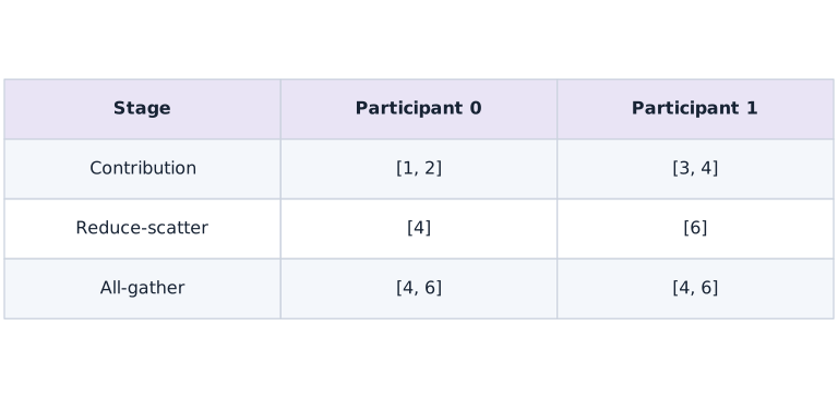
Contributions and are summed into portions and . After reduce-scatter neither participant holds the full result. All-gather then gives each . This analytic example shows ownership, not a physical schedule or measured traffic.
Keep normalization independent of device count
Our regression problem has sixteen observations and eight weights. Each of four devices receives four observations. Inside shard_map, the local function sees that local batch, but its gradient contribution still divides by the global count . Summing those contributions produces the derivative of the global mean loss. Dividing by the local count and summing would multiply the gradient by four. The NumPy expression calculates the complete derivative without JAX collectives.
Read the local result before interpreting the global array
Both programs return a global vector with shape . With all-reduce, each device holds all eight values; the output specification is P(). With reduce-scatter, each holds two consecutive values; P("data") describes how these pieces form the global vector. The full-array NumPy comparison checks values, while inspecting addressable shards checks storage. A shape print alone cannot distinguish these results.
Derive a communication model with its assumptions visible
Let be the byte size of one complete gradient and the number of ranks. In an idealized ring, reduce-scatter sends a total of bytes per rank. A subsequent all-gather sends the same amount. Their sum gives the usual two-phase ring all-reduce payload. For eight float32 values, bytes and : the modeled payloads are twenty-four and forty-eight bytes per rank. These are algorithmic payload counts, not measured traffic or total memory use. They omit latency, protocol overhead and topology.
Follow the consumer of the gradient
An elementwise optimizer can update matching parameter and momentum slices using a gradient slice. This can reduce persistent per-device optimizer storage. But if the next forward pass expects replicated weights, those updated weights still need gathering. Reducing one collective does not automatically reduce the communication of a whole training step.
Our example implements the gather explicitly and checks the reconstructed vector. In installed JAX 0.9.2, the default all_gather variation rule does not infer the replicated output required here. Only this small wrapper sets check_vma=False; its proof is that every rank gathers the same ordered slices. The code verifies every local replica as well as the global reference. Do not disable variation checks to conceal a genuinely rank-dependent output.
Separate observed execution from the payload model and run on a TPU mesh
The lowered StableHLO is inspected for the requested collective operations. The benchmark warms each exact function and waits for every result; it prints seven CPU timing samples summarized by their medians. Compilation is excluded. These logical devices share one host and do not reproduce a TPU network.
A reduce-scatter may time slower than an all-reduce on this tiny workload. That observation does not invalidate the byte calculation: timing also depends on dispatch, implementation and synchronization. The separate gather timing is an isolated call; summing isolated medians is not a measured fused training-step latency. Benchmark the complete consuming algorithm on its actual hardware before reporting a system improvement. When you run this lesson on a 4-chip TPU VM (v5litepod-4 or v6e-4) from the TPU course (phase-tpu), remove the CPU platform override so shard_map lowers psum and psum_scatter onto physical TPU ICI links.
Run all-reduce and reduce-scatter across 4 TPU chips on a TPU VM
gcloud compute tpus tpu-vm scp exercises/distributed-03.py $TPU_NAME:~/jax-tpu-lab/ --zone=$ZONE
gcloud compute tpus tpu-vm ssh $TPU_NAME --zone=$ZONE \
  --command="sed \"s/jax.config.update('jax_platforms', 'cpu')/# use default TPU backend/; s/jax.config.update('jax_num_cpu_devices', 4)/# use physical TPU chips/\" ~/jax-tpu-lab/distributed-03.py > ~/jax-tpu-lab/distributed-03-tpu.py && JAX_PLATFORMS=tpu ~/jax-tpu-lab/.venv/bin/python ~/jax-tpu-lab/distributed-03-tpu.py"
Expected:
Verifies that all_reduce, reduce_scatter, and all_gather match the NumPy reference across 4 physical TPU devices and prints completed TPU median microseconds.
One mathematical gradient, different local storage
Predict before looking: Will equal global gradients imply equal numbers of stored values on each device?
Read the figure
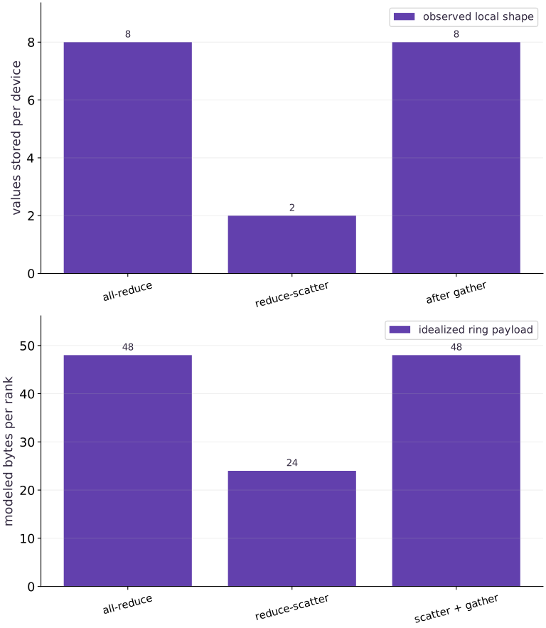
The upper panel counts values in one local result: eight for all-reduce, two for reduce-scatter, and eight after gathering. These counts come from actual addressable shards. All three global vectors contain the same eight gradient values. The lower panel shows the idealized ring payload in bytes per rank: forty-eight for all-reduce, twenty-four for reduce-scatter alone, and forty-eight when gathering is added. It is a model, not measured device traffic.
Connect it to the computation
The reduction in the middle storage bar comes from partitioning the summed gradient. The return of both bars after gathering explains why a local memory benefit and a complete communication benefit are different claims. The momentum experiment consumes slices before reconstructing weights. Its numerical comparison checks correctness; the separate synchronized CPU samples check a different question and is distinct from accelerator speed.
Open full-size figureDownload data and provenance
The notebook contains the data experiment, plotting code, and recorded figure output. Rerun it to test your changes.
Where to put & run this code: Work in phases/09-distributed/03-communication-efficient-algorithms/code/main.py (or downloaded exercises/distributed-03.py / exercises/distributed-03.ipynb) and execute from the repository root with python3 phases/09-distributed/03-communication-efficient-algorithms/code/main.py.
1 Configure four logical devices
Add this block after the preceding block in a fresh Python file, then run the complete file.
# Step 1 — Configure four logical devices: Compare both the numerical global result and the placement needed...
import jax
# Update state in place with the new values.
jax.config.update('jax_platforms', 'cpu')
# Update state in place with the new values.
jax.config.update('jax_num_cpu_devices', 4)
import jax.numpy as jnp
import numpy as np
from jax.sharding import Mesh, NamedSharding, PartitionSpec as P
from time import perf_counter
Code building blocks in this step
Mesh + PartitionSpec + NamedSharding— Maps logical tensor axes onto physical device mesh axes for SPMD data, tensor, or pipeline parallelism.
Compare both the numerical global result and the placement needed by its next consumer.
2 Place the data and model
Add this block after the preceding block in a fresh Python file, then run the complete file.
# Step 2 — Place the data and model: Compare both the numerical global result and the placement needed...
assert jax.local_device_count() == 4, 'Restart with four logical CPU devices'
# Configure multi-device placement / sharding specification (`mesh`).
mesh = Mesh(np.asarray(jax.devices()), ('data',))
# Configure multi-device placement / sharding specification (`rows`).
rows = NamedSharding(mesh, P('data', None))
# Configure multi-device placement / sharding specification (`replicated`).
replicated = NamedSharding(mesh, P())
# Configure multi-device placement / sharding specification (`features`).
features = NamedSharding(mesh, P('data'))
# Construct and reshape `xh` into the target tensor dimensions.
xh = np.arange(16 * 8, dtype=np.float32).reshape(16, 8) / 128 - 0.5
yh = xh @ np.linspace(-0.4, 0.3, 8, dtype=np.float32)
wh = np.linspace(0.1, -0.2, 8, dtype=np.float32)
# Place `x` explicitly onto the target JAX device.
x = jax.device_put(xh, rows)
# Configure multi-device placement / sharding specification (`y`).
y = jax.device_put(yh, NamedSharding(mesh, P('data')))
# Place `w` explicitly onto the target JAX device.
w = jax.device_put(wh, replicated)
Code building blocks in this step
array.reshape(new_shape)— Reorganizes tensor axes without changing the total element count (array.size).Mesh + PartitionSpec + NamedSharding— Maps logical tensor axes onto physical device mesh axes for SPMD data, tensor, or pipeline parallelism.
Compare both the numerical global result and the placement needed by its next consumer.
3 Implement partial gradients and collectives
Add this block after the preceding block in a fresh Python file, then run the complete file.
# Step 3 — Implement partial gradients and collectives: Compare both the numerical global result and the placement needed...
def local_contribution(a, b, weights):
    return 2 * a.T @ (a @ weights - b) / 16
Code building blocks in this step
local_contribution(...)— Calllocal_contributionwith your updated parameters or inputs from this lesson's workspace.
Compare both the numerical global result and the placement needed by its next consumer.
4 Verify the result and placement
Add this block after the preceding block in a fresh Python file, then run the complete file.
# Step 4 — Verify the result and placement: Compare both the numerical global result and the placement needed...
def reduce_all(a, b, weights):
    return jax.lax.psum(local_contribution(a, b, weights), 'data')
Code building blocks in this step
reduce_all(...)— Callreduce_allwith your updated parameters or inputs from this lesson's workspace.lax.psum(...)— Calllax.psumwith your updated parameters or inputs from this lesson's workspace.
Compare both the numerical global result and the placement needed by its next consumer.
5 Measure completed calls
Add this block after the preceding block in a fresh Python file, then run the complete file.
# Step 5 — Measure completed calls: Compare both the numerical global result and the placement needed...
def reduce_shard(a, b, weights):
    return jax.lax.psum_scatter(local_contribution(a, b, weights), 'data', tiled=True)
Code building blocks in this step
reduce_shard(...)— Callreduce_shardwith your updated parameters or inputs from this lesson's workspace.lax.psum_scatter(...)— Calllax.psum_scatterwith your updated parameters or inputs from this lesson's workspace.
Compare both the numerical global result and the placement needed by its next consumer.
6 Measure completed calls
Add this block after the preceding block in a fresh Python file, then run the complete file.
# Step 6 — Measure completed calls: Compare both the numerical global result and the placement needed...
# Configure multi-device placement / sharding specification (`all_gradient`).
all_gradient = jax.jit(jax.shard_map(reduce_all, mesh=mesh,
    in_specs=(P('data', None), P('data'), P()), out_specs=P()))
# Configure multi-device placement / sharding specification (`shard_gradient`).
shard_gradient = jax.jit(jax.shard_map(reduce_shard, mesh=mesh,
    in_specs=(P('data', None), P('data'), P()), out_specs=P('data')))
# Configure multi-device placement / sharding specification (`gather`).
gather = jax.jit(jax.shard_map(lambda g: jax.lax.all_gather(g, 'data', tiled=True),
    mesh=mesh, in_specs=P('data'), out_specs=P(), check_vma=False))
ga = all_gradient(x, y, w)
gs = shard_gradient(x, y, w)
gg = gather(gs)
reference = 2 * xh.T @ (xh @ wh - yh) / 16
for result in [ga, gs, gg]:
    # Convert `` to a host NumPy array for inspection or verification.
    np.testing.assert_allclose(np.asarray(result), reference, atol=2e-6, rtol=2e-6)
# Check tensor shape invariant: `all(s.data.shape == (8,) for s in ga.addressable_shards)`
assert all(s.data.shape == (8,) for s in ga.addressable_shards)
# Check tensor shape invariant: `all(s.data.shape == (2,) for s in gs.addressable_shards)`
assert all(s.data.shape == (2,) for s in gs.addressable_shards)
# Check tensor shape invariant: `all(s.data.shape == (8,) for s in gg.addressable_shards)`
assert all(s.data.shape == (8,) for s in gg.addressable_shards)
# Trace or lower the function to inspect its compiler representation (`hlo_all`).
hlo_all = str(all_gradient.lower(x, y, w).compiler_ir(dialect='stablehlo'))
hlo_shard = str(shard_gradient.lower(x, y, w).compiler_ir(dialect='stablehlo'))
assert 'all_reduce' in hlo_all and 'reduce_scatter' in hlo_shard
Code building blocks in this step
jnp.allclose(actual, expected, rtol=..., atol=...)— Checks that two arrays match elementwise within floating-point tolerance.jax.jit(fn) / @jax.jit— Tracesfnwith abstract shapes and compiles a fused XLA executable cached by input shape and dtype.Mesh + PartitionSpec + NamedSharding— Maps logical tensor axes onto physical device mesh axes for SPMD data, tensor, or pipeline parallelism.
Compare both the numerical global result and the placement needed by its next consumer.
7 Measure completed calls
Add this block after the preceding block in a fresh Python file, then run the complete file.
# Step 7 — Measure completed calls: Compare both the numerical global result and the placement needed...
def completed_samples(fn, *args):
    # Synchronize host execution until asynchronous device computation completes.
    fn(*args).block_until_ready()
    samples = []
    for _ in range(7):
        start = perf_counter()
        # Synchronize host execution until asynchronous device computation completes.
        fn(*args).block_until_ready()
        samples.append((perf_counter() - start) * 1e6)
    return samples
all_us = completed_samples(all_gradient, x, y, w)
shard_us = completed_samples(shard_gradient, x, y, w)
gather_us = completed_samples(gather, gs)
# Idealized ring payload per rank; not a network measurement.
ranks, gradient_bytes = 4, wh.nbytes
ring_scatter_bytes = (ranks - 1) / ranks * gradient_bytes
ring_all_bytes = 2 * ring_scatter_bytes
print('Gradient reference:', reference.tolist())
print('Local result shapes: replicated (8,), reduce-scatter (2,), gathered (8,)')
print('Idealized ring bytes per rank:', ring_all_bytes, ring_scatter_bytes)
print('Completed CPU median microseconds:', {
    'all_reduce': float(np.median(all_us)), 'reduce_scatter': float(np.median(shard_us)),
    'all_gather_only': float(np.median(gather_us))})
Code building blocks in this step
jax.block_until_ready(output)— Synchronizes with the accelerator/CPU device so asynchronous dispatch finishes before wall-clock timing.
Compare both the numerical global result and the placement needed by its next consumer.
View the cumulative build in main.py
These blocks append in order to the same file.
# Step 1 — Configure four logical devices: Compare both the numerical global result and the placement needed...
import jax
# Update state in place with the new values.
jax.config.update('jax_platforms', 'cpu')
# Update state in place with the new values.
jax.config.update('jax_num_cpu_devices', 4)
import jax.numpy as jnp
import numpy as np
from jax.sharding import Mesh, NamedSharding, PartitionSpec as P
from time import perf_counter

# Step 2 — Place the data and model: Compare both the numerical global result and the placement needed...
assert jax.local_device_count() == 4, 'Restart with four logical CPU devices'
# Configure multi-device placement / sharding specification (`mesh`).
mesh = Mesh(np.asarray(jax.devices()), ('data',))
# Configure multi-device placement / sharding specification (`rows`).
rows = NamedSharding(mesh, P('data', None))
# Configure multi-device placement / sharding specification (`replicated`).
replicated = NamedSharding(mesh, P())
# Configure multi-device placement / sharding specification (`features`).
features = NamedSharding(mesh, P('data'))
# Construct and reshape `xh` into the target tensor dimensions.
xh = np.arange(16 * 8, dtype=np.float32).reshape(16, 8) / 128 - 0.5
yh = xh @ np.linspace(-0.4, 0.3, 8, dtype=np.float32)
wh = np.linspace(0.1, -0.2, 8, dtype=np.float32)
# Place `x` explicitly onto the target JAX device.
x = jax.device_put(xh, rows)
# Configure multi-device placement / sharding specification (`y`).
y = jax.device_put(yh, NamedSharding(mesh, P('data')))
# Place `w` explicitly onto the target JAX device.
w = jax.device_put(wh, replicated)

# Step 3 — Implement partial gradients and collectives: Compare both the numerical global result and the placement needed...
def local_contribution(a, b, weights):
    return 2 * a.T @ (a @ weights - b) / 16

# Step 4 — Verify the result and placement: Compare both the numerical global result and the placement needed...
def reduce_all(a, b, weights):
    return jax.lax.psum(local_contribution(a, b, weights), 'data')

# Step 5 — Measure completed calls: Compare both the numerical global result and the placement needed...
def reduce_shard(a, b, weights):
    return jax.lax.psum_scatter(local_contribution(a, b, weights), 'data', tiled=True)

# Step 6 — Measure completed calls: Compare both the numerical global result and the placement needed...
# Configure multi-device placement / sharding specification (`all_gradient`).
all_gradient = jax.jit(jax.shard_map(reduce_all, mesh=mesh,
    in_specs=(P('data', None), P('data'), P()), out_specs=P()))
# Configure multi-device placement / sharding specification (`shard_gradient`).
shard_gradient = jax.jit(jax.shard_map(reduce_shard, mesh=mesh,
    in_specs=(P('data', None), P('data'), P()), out_specs=P('data')))
# Configure multi-device placement / sharding specification (`gather`).
gather = jax.jit(jax.shard_map(lambda g: jax.lax.all_gather(g, 'data', tiled=True),
    mesh=mesh, in_specs=P('data'), out_specs=P(), check_vma=False))
ga = all_gradient(x, y, w)
gs = shard_gradient(x, y, w)
gg = gather(gs)
reference = 2 * xh.T @ (xh @ wh - yh) / 16
for result in [ga, gs, gg]:
    # Convert `` to a host NumPy array for inspection or verification.
    np.testing.assert_allclose(np.asarray(result), reference, atol=2e-6, rtol=2e-6)
# Check tensor shape invariant: `all(s.data.shape == (8,) for s in ga.addressable_shards)`
assert all(s.data.shape == (8,) for s in ga.addressable_shards)
# Check tensor shape invariant: `all(s.data.shape == (2,) for s in gs.addressable_shards)`
assert all(s.data.shape == (2,) for s in gs.addressable_shards)
# Check tensor shape invariant: `all(s.data.shape == (8,) for s in gg.addressable_shards)`
assert all(s.data.shape == (8,) for s in gg.addressable_shards)
# Trace or lower the function to inspect its compiler representation (`hlo_all`).
hlo_all = str(all_gradient.lower(x, y, w).compiler_ir(dialect='stablehlo'))
hlo_shard = str(shard_gradient.lower(x, y, w).compiler_ir(dialect='stablehlo'))
assert 'all_reduce' in hlo_all and 'reduce_scatter' in hlo_shard

# Step 7 — Measure completed calls: Compare both the numerical global result and the placement needed...
def completed_samples(fn, *args):
    # Synchronize host execution until asynchronous device computation completes.
    fn(*args).block_until_ready()
    samples = []
    for _ in range(7):
        start = perf_counter()
        # Synchronize host execution until asynchronous device computation completes.
        fn(*args).block_until_ready()
        samples.append((perf_counter() - start) * 1e6)
    return samples
all_us = completed_samples(all_gradient, x, y, w)
shard_us = completed_samples(shard_gradient, x, y, w)
gather_us = completed_samples(gather, gs)
# Idealized ring payload per rank; not a network measurement.
ranks, gradient_bytes = 4, wh.nbytes
ring_scatter_bytes = (ranks - 1) / ranks * gradient_bytes
ring_all_bytes = 2 * ring_scatter_bytes
print('Gradient reference:', reference.tolist())
print('Local result shapes: replicated (8,), reduce-scatter (2,), gathered (8,)')
print('Idealized ring bytes per rank:', ring_all_bytes, ring_scatter_bytes)
print('Completed CPU median microseconds:', {
    'all_reduce': float(np.median(all_us)), 'reduce_scatter': float(np.median(shard_us)),
    'all_gather_only': float(np.median(gather_us))})
Run the example
python3 phases/09-distributed/03-communication-efficient-algorithms/code/main.pyAbout this command
This shortcut uses an activated macOS/Linux course environment in the repository folder. For Windows, use the explicit interpreter command in “Setup help” above. The script includes worked examples and reference solutions.
Inspect the complete assembled example
# Step 1 — Configure four logical devices: Compare both the numerical global result and the placement needed...
import jax
# Update state in place with the new values.
jax.config.update('jax_platforms', 'cpu')
# Update state in place with the new values.
jax.config.update('jax_num_cpu_devices', 4)
import jax.numpy as jnp
import numpy as np
from jax.sharding import Mesh, NamedSharding, PartitionSpec as P
from time import perf_counter

# Step 2 — Place the data and model: Compare both the numerical global result and the placement needed...
assert jax.local_device_count() == 4, 'Restart with four logical CPU devices'
# Configure multi-device placement / sharding specification (`mesh`).
mesh = Mesh(np.asarray(jax.devices()), ('data',))
# Configure multi-device placement / sharding specification (`rows`).
rows = NamedSharding(mesh, P('data', None))
# Configure multi-device placement / sharding specification (`replicated`).
replicated = NamedSharding(mesh, P())
# Configure multi-device placement / sharding specification (`features`).
features = NamedSharding(mesh, P('data'))
# Construct and reshape `xh` into the target tensor dimensions.
xh = np.arange(16 * 8, dtype=np.float32).reshape(16, 8) / 128 - 0.5
yh = xh @ np.linspace(-0.4, 0.3, 8, dtype=np.float32)
wh = np.linspace(0.1, -0.2, 8, dtype=np.float32)
# Place `x` explicitly onto the target JAX device.
x = jax.device_put(xh, rows)
# Configure multi-device placement / sharding specification (`y`).
y = jax.device_put(yh, NamedSharding(mesh, P('data')))
# Place `w` explicitly onto the target JAX device.
w = jax.device_put(wh, replicated)

# Step 3 — Implement partial gradients and collectives: Compare both the numerical global result and the placement needed...
def local_contribution(a, b, weights):
    return 2 * a.T @ (a @ weights - b) / 16

# Step 4 — Verify the result and placement: Compare both the numerical global result and the placement needed...
def reduce_all(a, b, weights):
    return jax.lax.psum(local_contribution(a, b, weights), 'data')

# Step 5 — Measure completed calls: Compare both the numerical global result and the placement needed...
def reduce_shard(a, b, weights):
    return jax.lax.psum_scatter(local_contribution(a, b, weights), 'data', tiled=True)

# Step 6 — Measure completed calls: Compare both the numerical global result and the placement needed...
# Configure multi-device placement / sharding specification (`all_gradient`).
all_gradient = jax.jit(jax.shard_map(reduce_all, mesh=mesh,
    in_specs=(P('data', None), P('data'), P()), out_specs=P()))
# Configure multi-device placement / sharding specification (`shard_gradient`).
shard_gradient = jax.jit(jax.shard_map(reduce_shard, mesh=mesh,
    in_specs=(P('data', None), P('data'), P()), out_specs=P('data')))
# Configure multi-device placement / sharding specification (`gather`).
gather = jax.jit(jax.shard_map(lambda g: jax.lax.all_gather(g, 'data', tiled=True),
    mesh=mesh, in_specs=P('data'), out_specs=P(), check_vma=False))
ga = all_gradient(x, y, w)
gs = shard_gradient(x, y, w)
gg = gather(gs)
reference = 2 * xh.T @ (xh @ wh - yh) / 16
for result in [ga, gs, gg]:
    # Convert `` to a host NumPy array for inspection or verification.
    np.testing.assert_allclose(np.asarray(result), reference, atol=2e-6, rtol=2e-6)
# Check tensor shape invariant: `all(s.data.shape == (8,) for s in ga.addressable_shards)`
assert all(s.data.shape == (8,) for s in ga.addressable_shards)
# Check tensor shape invariant: `all(s.data.shape == (2,) for s in gs.addressable_shards)`
assert all(s.data.shape == (2,) for s in gs.addressable_shards)
# Check tensor shape invariant: `all(s.data.shape == (8,) for s in gg.addressable_shards)`
assert all(s.data.shape == (8,) for s in gg.addressable_shards)
# Trace or lower the function to inspect its compiler representation (`hlo_all`).
hlo_all = str(all_gradient.lower(x, y, w).compiler_ir(dialect='stablehlo'))
hlo_shard = str(shard_gradient.lower(x, y, w).compiler_ir(dialect='stablehlo'))
assert 'all_reduce' in hlo_all and 'reduce_scatter' in hlo_shard

# Step 7 — Measure completed calls: Compare both the numerical global result and the placement needed...
def completed_samples(fn, *args):
    # Synchronize host execution until asynchronous device computation completes.
    fn(*args).block_until_ready()
    samples = []
    for _ in range(7):
        start = perf_counter()
        # Synchronize host execution until asynchronous device computation completes.
        fn(*args).block_until_ready()
        samples.append((perf_counter() - start) * 1e6)
    return samples
all_us = completed_samples(all_gradient, x, y, w)
shard_us = completed_samples(shard_gradient, x, y, w)
gather_us = completed_samples(gather, gs)
# Idealized ring payload per rank; not a network measurement.
ranks, gradient_bytes = 4, wh.nbytes
ring_scatter_bytes = (ranks - 1) / ranks * gradient_bytes
ring_all_bytes = 2 * ring_scatter_bytes
print('Gradient reference:', reference.tolist())
print('Local result shapes: replicated (8,), reduce-scatter (2,), gathered (8,)')
print('Idealized ring bytes per rank:', ring_all_bytes, ring_scatter_bytes)
print('Completed CPU median microseconds:', {
    'all_reduce': float(np.median(all_us)), 'reduce_scatter': float(np.median(shard_us)),
    'all_gather_only': float(np.median(gather_us))})
Expected result: All three global gradients agree with NumPy. The replicated and reconstructed local results contain eight values each; reduce-scatter shards contain two. The idealized ring payload is 48 bytes per rank for all-reduce and 24 for reduce-scatter. Actual CPU timing samples vary.
Recorded reference execution
Reference output captured from executing the complete lesson script (code/main.py) and its assertions in the course CPU environment.
Gradient reference: [0.0029296851716935635, 0.00219726306386292, 0.0014648411888629198, 0.0007324193138629198, -2.6193447411060333e-09, -0.000732424552552402, -0.001464846427552402, -0.002197268418967724]
Local result shapes: replicated (8,), reduce-scatter (2,), gathered (8,)
Idealized ring bytes per rank: 48.0 24.0
Completed CPU median microseconds: {'all_reduce': 99.08340871334076, 'reduce_scatter': 102.49996557831764, 'all_gather_only': 108.41712355613708}
Gradient reference: [0.0029296851716935635, 0.00219726306386292, 0.0014648411888629198, 0.0007324193138629198, -2.6193447411060333e-09, -0.000732424552552402, -0.001464846427552402, -0.002197268418967724]
Local result shapes: replicated (8,), reduce-scatter (2,), gathered (8,)
Idealized ring bytes per rank: 48.0 24.0
Completed CPU median microseconds: {'all_reduce': 109.4592735171318, 'reduce_scatter': 109.74984616041183, 'all_gather_only': 86.12498641014099}
Sharded momentum matches the independent elementwise update.
Joint permutation preserves the gradient; label-only reversal does not.
Idealized payload/storage budget, not observed network traffic: [{'ranks': 2, 'all_reduce_bytes': 1048576, 'scatter_gather_bytes': 1048576, 'shard_storage_bytes': 524288}, {'ranks': 4, 'all_reduce_bytes': 1572864, 'scatter_gather_bytes': 1572864, 'shard_storage_bytes': 262144}, {'ranks': 8, 'all_reduce_bytes': 1835008, 'scatter_gather_bytes': 1835008, 'shard_storage_bytes': 131072}]
PASS: distributed-03
Download execution record · The notebook includes executed cells and figure outputs. Compare your run with these values; timings depend on the machine.
Update slices before gathering
# Experiment — Update slices before gathering: An elementwise update can consume the partitioned gradient.
v_host = np.linspace(-0.02, 0.03, 8, dtype=np.float32)
# Place `ws` explicitly onto the target JAX device.
ws = jax.device_put(wh, features)
# Place `vs` explicitly onto the target JAX device.
vs = jax.device_put(v_host, features)
new_v = 0.9 * vs + gs
new_w = ws - 0.1 * new_v
updated = gather(new_w)
expected_w = wh - 0.1 * (0.9 * v_host + reference)
# Convert `` to a host NumPy array for inspection or verification.
np.testing.assert_allclose(np.asarray(updated), expected_w, atol=2e-6, rtol=2e-6)
for shard in updated.addressable_shards:
    # Convert `` to a host NumPy array for inspection or verification.
    np.testing.assert_allclose(np.asarray(shard.data), expected_w, atol=2e-6, rtol=2e-6)
# Check tensor shape invariant: `all(s.data.shape == (2,) for s in new_v.addressable_shards)`
assert all(s.data.shape == (2,) for s in new_v.addressable_shards)
print('Sharded momentum matches the independent elementwise update.')
Expected: The gathered update matches the independent momentum formula, while local momentum retains two values.
An elementwise update can consume the partitioned gradient. Gathering the updated parameter later is still real communication, so include it when evaluating the full algorithm.
Make it yours
Where to put your code: Append your solution at the bottom of phases/09-distributed/03-communication-efficient-algorithms/code/main.py (or inside the Make it yours cell of exercises/distributed-03.ipynb) and run python3 phases/09-distributed/03-communication-efficient-algorithms/code/main.py to verify your prediction before opening the reference solution.
Repeat the gradient comparison after reversing both observation rows and labels and changing the initial weights. Verify every all-reduce and reconstructed local replica, then explain why reversing only the labels changes the problem.
Show a writing guide and starter scaffold
How to write this exercise code: step-by-step recipe & starter scaffold
1. Key functions & syntax to use:
jnp.allclose(actual, expected, rtol=..., atol=...)— Checks that two arrays match elementwise within floating-point tolerance.Mesh + PartitionSpec + NamedSharding— Maps logical tensor axes onto physical device mesh axes for SPMD data, tensor, or pipeline parallelism.
2. Step-by-step implementation plan:
- Configure multi-device placement / sharding specification (
y2). - Place
w2explicitly onto the target JAX device. - Convert
to a host NumPy array for inspection or verification. - Convert
to a host NumPy array for inspection or verification.
# Exercise solution: Repeat the gradient comparison after reversing both observation rows...
x2 = jax.device_put(...)  # TODO: compute x2
# Configure multi-device placement / sharding specification (`y2`).
y2 = jax.device_put(...)  # TODO: compute y2
w2h = ...  # TODO: compute w2h
# Place `w2` explicitly onto the target JAX device.
w2 = jax.device_put(...)  # TODO: compute w2
r2 = ...  # TODO: compute r2
for answer in [all_gradient(x2, y2, w2), gather(shard_gradient(x2, y2, w2))]:
    # Convert `` to a host NumPy array for inspection or verification.
    np.testing.assert_allclose(np.asarray(answer), r2, atol = ...  # TODO: compute np.testing.assert_allclose(np.asarray(answer), r2, atol
    for shard in answer.addressable_shards:
        # Convert `` to a host NumPy array for inspection or verification.
        np.testing.assert_allclose(np.asarray(shard.data), r2, atol = ...  # TODO: compute np.testing.assert_allclose(np.asarray(shard.data), r2, atol
wrong_labels = ...  # TODO: compute wrong_labels
assert np.max(np.abs(wrong_labels-r2))  # TODO: complete assertion check
print('Joint permutation preserves the gradient; label-only reversal does not.')
Reveal the reference solution
# Exercise solution: Repeat the gradient comparison after reversing both observation rows...
x2 = jax.device_put(xh[::-1].copy(), rows)
# Configure multi-device placement / sharding specification (`y2`).
y2 = jax.device_put(yh[::-1].copy(), NamedSharding(mesh, P('data')))
w2h = wh + np.float32(0.17)
# Place `w2` explicitly onto the target JAX device.
w2 = jax.device_put(w2h, replicated)
r2 = 2 * xh.T @ (xh @ w2h - yh) / 16
for answer in [all_gradient(x2, y2, w2), gather(shard_gradient(x2, y2, w2))]:
    # Convert `` to a host NumPy array for inspection or verification.
    np.testing.assert_allclose(np.asarray(answer), r2, atol=2e-6, rtol=2e-6)
    for shard in answer.addressable_shards:
        # Convert `` to a host NumPy array for inspection or verification.
        np.testing.assert_allclose(np.asarray(shard.data), r2, atol=2e-6, rtol=2e-6)
wrong_labels = 2 * xh.T @ (xh @ w2h - yh[::-1]) / 16
assert np.max(np.abs(wrong_labels-r2)) > 0.01
print('Joint permutation preserves the gradient; label-only reversal does not.')
Account for the complete communication cycle
Transfer
Compare a complete ring all-reduce with reduce-scatter followed by all-gather for a gradient of one mebibyte at two, four and eight ranks. Also compute per-rank gradient storage. Explain why lower storage does not guarantee fewer communicated bytes.
Show a writing guide and starter scaffold
How to write this practice solution: step-by-step recipe & starter scaffold
1. Key functions & syntax to use:
cycle(...)— Callcyclewith your updated parameters or inputs from this lesson's workspace.budget.append(...)— Callbudget.appendwith your updated parameters or inputs from this lesson's workspace.assert condition— Verify that the observed output shape, status, or numerical value satisfies the contract.
2. Step-by-step implementation plan:
- Set up the changed input or configuration parameters requested in the prompt.
- Run the target function or transformation and assert that the output matches your prediction.
# Account for the complete communication cycle (Transfer): The two-phase payload equals the all-reduce payload under...
budget = ...  # TODO: compute budget
for p in [2, 4, 8]:
    size = ...  # TODO: compute size
    rs = ...  # TODO: compute rs
    ar = ...  # TODO: compute ar
    cycle = ...  # TODO: compute cycle
    assert ar  # TODO: complete assertion check
    assert size // p * p  # TODO: complete assertion check
    budget.append({'ranks': p, 'all_reduce_bytes': ar,
                   'scatter_gather_bytes': cycle, 'shard_storage_bytes': size // p})
assert [row['all_reduce_bytes'] for row  # TODO: complete assertion check
print('Idealized payload/storage budget, not observed network traffic:', budget)
Show a hint
Use the same full gradient byte count for both collectives; one mebibyte is 2**20 bytes. Divide storage by ranks only for the sharded state.
Reveal reference solution and reasoning
# Account for the complete communication cycle (Transfer): The two-phase payload equals the all-reduce payload under...
budget = []
for p in [2, 4, 8]:
    size = 2**20
    rs = size * (p - 1) // p
    ar = 2 * rs
    cycle = rs + rs
    assert ar == cycle
    assert size // p * p == size
    budget.append({'ranks': p, 'all_reduce_bytes': ar,
                   'scatter_gather_bytes': cycle, 'shard_storage_bytes': size // p})
assert [row['all_reduce_bytes'] for row in budget] == [1048576, 1572864, 1835008]
print('Idealized payload/storage budget, not observed network traffic:', budget)
The two-phase payload equals the all-reduce payload under this model, even though the persistent sharded state is smaller. Timing and algorithm selection still need measurements on the complete target workload.
Diagnose the result
A gradient four times too large suggests local-mean normalization was summed. Correct global values with wrong local shapes suggest an output placement mismatch. A variation error in a replicated output needs a mathematical replication argument before changing the check.
Carry forward
- Check both global values and local storage.
- Derive collective costs for the complete consumer path.
- Label ring payload arithmetic separately from measured CPU timing.
Keep your evidence
Keep global NumPy gradient checks, local shard shapes, lowered collectives, changed-value replicas and complete scatter/gather payload accounting. Separate the idealized ring model from observed CPU timings.
Save your modified code, its output, and an explanation of your prediction. Checkpoint answers and exercise evidence are tracked separately.
Saved in this browser. Export or back up your portfolio anytime in My learning.
Verified on local CPU. Stage to a Cloud TPU VM via Cloud TPU setup to record accelerator execution receipts (TODO: add automated Cloud TPU CI execution receipts).