 JAX Pathways
Phase 14 / Autodiff & JAX internals
Read your first jaxpr
Revision v0.7.0 · Updated since your last visit. Review the changes; your progress is saved.
Lesson · about 90 minutes · CPU practice
Inspect a small transformed function and identify its operations.
Phase study guide: preparation, milestones and project evidence
Before you start
Before this: Math & optimization
Hardware: CPU
Setup help: Python, notebook, or Cloud TPU VM
Use the tested CPU packages (the recorded environment uses Python 3.14.3). Other Python versions and accelerator environments require separate checks. The optional Cloud TPU specialization explains the target-specific execution boundaries. Logical CPU devices practice partitioning; they do not simulate TPU performance.
Download the repository ZIP or use your existing checkout. Extract it and open a terminal in the folder containing requirements-cpu.txt. The beginner ZIP is separate; these lessons use the full repository folder.
python3 -m venv .venv
source .venv/bin/activate
python -m pip install -r requirements-cpu.txtpy -3 -m venv .venv
.\.venv\Scripts\python.exe -m pip install -r requirements-cpu.txtAfter activation, run the complete worked example from that same folder:
python phases/14-internals/01-read-your-first-jaxpr/code/main.py.\.venv\Scripts\python.exe phases/14-internals/01-read-your-first-jaxpr/code/main.pyFor an incremental build, create main.py in your own practice folder, append each build block in order, and run python main.py with this environment active. Keep that file separate from the downloaded reference solution.
Download this lesson’s notebook. Open it with a Python kernel using the course environment. Run cells from the top after restarting the kernel; experiments depend on earlier definitions.
For local Jupyter, first install the course requirements using the Local Python steps, then use your environment’s Python to start Jupyter:
python -m pip install jupyterlab
python -m jupyter lab.\.venv\Scripts\python.exe -m pip install jupyterlab
.\.venv\Scripts\python.exe -m jupyter labSelect the downloaded internals-01.ipynb file in JupyterLab. The notebook contains reference solutions; make your prediction and attempt each practice task before opening them. Restart the kernel before changing logical device setup.
The worked reference for this lesson is CPU-validated. Some references explicitly configure logical CPU devices; setting JAX_PLATFORMS does not adapt them to a TPU. Follow the execution matrix and reviewed multi-host example before attempting a target run.
For accelerator preparation, study TPU setup, observed runtime receipts, checkpointed jobs and precision and retained traces. These target paths remain unqualified on physical TPU hardware until an actual receipt is recorded. Cloud provisioning is optional for CPU learning.
Check: Forward operations include add, mul and reduce_sum, with output shapes , , (). Value: ; gradient: . Variable names and printed primitive parameters may vary by JAX version.
Revisit the guided CPU setup · Open 19: TPU Setup. Package instructions are CPU instructions; Windows and accelerator environments need their own validation.
What you will be able to do
- Translate jaxpr variables and array types into a data-flow diagram.
- Compare a forward computation with its gradient program.
- Distinguish a closed-over array constant from a function input.
- Diagnose a traced Python branch and verify a lax.cond repair.
- Compare an unrolled loop with a scan without claiming a speedup.
The problem
Your function returns the right answer. Now let’s look inside the computation JAX traced. We’ll start with three operations, calculate each intermediate value ourselves, and match them to a jaxpr. Then we’ll see what changes after differentiation. The printed representation is a learning tool, not a measurement of execution speed.
The idea
A jaxpr records primitive operations and the values that connect them. Read it as a data-flow program with shapes and dtypes, not as a literal description of final hardware instructions or Python execution order.
Read a jaxpr as a typed computation
Start at the inputs and trace one intermediate to its consumers. For a reduction, identify the consumed axes and resulting shape. Distinguish array inputs from closed constants: both can affect the output, but they enter the program differently.
Then connect each primitive to the corresponding part of the original expression. A variable name in a printed jaxpr is a local label, not a stable API to test verbatim.
The intermediate-value heatmap is a numerical aid. Pair it with the typed dependency graph to explain how those values were produced. Lowering and compilation can change representation later; a primitive count alone does not predict executed kernel count or runtime.
Compute the values before reading the representation
Start with . Adding gives . Elementwise multiplication of this vector by itself gives . The sum is . The first two operations retain shape , while the reduction produces a scalar, whose array shape is ().
The derivative of each is , so the gradient at this input is . A different implementation could produce the same values with different primitives. We use multiplication explicitly to keep this first trace readable. Do not infer an algorithm from the spelling of a Python expression alone.
x: f32[3] = [1, 2, 3]
   │ add scalar 1
   ▼
shifted: f32[3] = [2, 3, 4]
   │ multiply by shifted
   ▼
squared: f32[3] = [4, 9, 16]
   │ reduce_sum over axis 0
   ▼
result: f32[] = 29
Read one equation at a time
In a typical printout the input is named a, the shifted vector b, the squared vector c, and the scalar result . These names are generated; they are not your Python variable names and can change across versions. An equation such as b:f32[3] = add a 1.0:f32[] binds a new value rather than mutating a. f32 means float32, denotes a length-three vector, and [] denotes a scalar.
The lambda header lists closed constants before its semicolon and ordinary input variables after it. The let block lists equations; the final in (...) lists returned values. Parameters in brackets belong to a primitive, for example reduction axes. Our script iterates over eqns and prints primitive names and output shapes so you can relate the structured object to the text. Treat exact formatting and generated names as version-dependent details.
{ lambda ; a:f32[3]. let
    b:f32[3] = add a 1.0:f32[]
    c:f32[3] = mul b b
    d:f32[] = reduce_sum[...] c
  in (d,) }
Illustrative excerpt: actual reduction parameters may differ.
Trace an abstract signature, not the sample’s values
make_jaxpr uses an example array to establish an abstract input shape and dtype. It does not use the ordinary data values as Python control-flow decisions. Calling the same function with another float32 length-three array follows the same computation structure. A length-four input changes the types in the representation, even though the algorithm is still add, multiply, sum.
This is why if > cannot select a Python branch during ordinary tracing: the comparison produces a traced boolean, not a concrete Python truth value. Use array-compatible control flow such as lax.cond with compatible branch result types. Moving the predicate into a static argument is a different design and may trigger separate traces; it is not a universal repair.
Inspect the gradient as another program
make_jaxpr(grad(shifted_square_sum))(x) asks JAX to trace the transformed derivative function. You will see additional operations that propagate a scalar output sensitivity back to vector inputs, including multiplication and broadcasting. Some forward operations may remain; their exact arrangement depends on transformations and JAX’s implementation.
Count the equations as a descriptive observation, then verify the numerical derivative independently at multiple inputs. More equations do not automatically mean slower execution: lowering, fusion, memory movement and hardware scheduling affect runtime. A jaxpr can tell you what was traced; profiling answers where time is spent.
Separate data inputs from captured constants
An array defined outside a function and read by it can appear as a closed constant. In the exercise below the offset vector is ; remains the ordinary input. Inspect closed.consts and jaxpr.constvars, then compare with a version that takes the offset as an explicit second argument. The explicit version has two input variables.
This distinction matters for clarity and reusable function signatures. It does not prove that a constant occupies a particular device memory buffer or is copied on every call. Later compiler stages can represent constants differently. Save the traced structure without presenting it as a memory trace.
Compare Python unrolling with structured iteration
A Python loop with a fixed range is executed during tracing, so its repeated array operations can appear repeatedly in the outer jaxpr. lax.scan represents a loop with a nested body and a carry contract; the outer equation list includes the loop primitive rather than simply expanding every iteration.
Inspect both representations for a four-step recurrence and verify they return the same result. The body jaxpr still contains operations, so counting only outer equations would hide work. This comparison illustrates representation, not a benchmark. For an actual performance claim, measure compilation and synchronized execution separately on the intended hardware.
Follow values through the jaxpr operations
Predict before looking: Which operation reduces an array to one scalar?
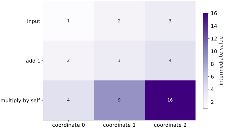
Read the figure
Columns track the three array coordinates, while rows track stages of a computation. The first row is input . Adding produces , and multiplying those values by themselves produces .
Follow one column downward: the final coordinate changes from to to . Its darker bottom cell reflects a larger intermediate value, not a more expensive operation or longer runtime.
Connect it to the computation
The final reduction adds the bottom row to obtain . That scalar is not another row in the heatmap because it no longer has three separate coordinates. This change of shape connects the elementwise operations to the reduction in the jaxpr.
A jaxpr describes operations and abstract values. The figure supplies concrete intermediate values for this one input, making that program easier to trace by hand. Changing the input changes these numbers without necessarily changing the jaxpr’s structure.
Open full-size figureDownload data and provenance
The notebook contains the data experiment, plotting code, and recorded figure output. Rerun it to test your changes.
Where to put & run this code: Work in phases/14-internals/01-read-your-first-jaxpr/code/main.py (or downloaded exercises/internals-01.py / exercises/internals-01.ipynb) and execute from the repository root with python3 phases/14-internals/01-read-your-first-jaxpr/code/main.py.
1 Establish the input signature
Create main.py in the activated setup environment and add the imports and float32 vector below. Calculate → → on paper.
# Step 1 — 1. Establish the input signature: The vector has shape (3,) and dtype float32; these determine the...
import jax
import jax.numpy as jnp

x = jnp.array([1., 2., 3.], dtype=jnp.float32)
Code building blocks in this step
jnp.array(values, dtype=...)— Constructs an immutable device-backed JAX array from Python/NumPy values.
The vector has shape and dtype float32; these determine the abstract input type.
2 Write the pure function
Append this function. It reads its argument and returns one scalar; no global mutation or Python branch is involved.
# Step 2 — 2. Write the pure function: Each assignment names a new value.
def shifted_square_sum(x):
    shifted = x + 1.
    squared = shifted * shifted
    return jnp.sum(squared)
Code building blocks in this step
x.sum(axis=...) / x.mean(axis=..., keepdims=...)— Reduces values along the namedaxis(the axis you name is collapsed unlesskeepdims=True).
Each assignment names a new value. sum reduces the three squared values to a scalar.
3 Inspect and independently verify
Append this block and run python main.py. Match each printed operation to the flow above, then compare the assertions with your paper calculation.
# Step 3 — 3. Inspect and independently verify: Forward operations include add, mul and reduce_sum, with output...
# Trace or lower the function to inspect its compiler representation (`closed`).
closed = jax.make_jaxpr(shifted_square_sum)(x)
print("Forward program:")
print(closed)
for equation in closed.jaxpr.eqns:
    print("Operation:", equation.primitive.name,
          "output shapes:", [v.aval.shape for v in equation.outvars])
value = shifted_square_sum(x)
# Differentiate the objective to obtain `gradient` via automatic differentiation.
gradient = jax.grad(shifted_square_sum)(x)
print("Value / gradient:", value, gradient)
assert jnp.allclose(value, 29.)
assert jnp.allclose(gradient, jnp.array([4., 6., 8.]))
Code building blocks in this step
jnp.array(values, dtype=...)— Constructs an immutable device-backed JAX array from Python/NumPy values.jnp.allclose(actual, expected, rtol=..., atol=...)— Checks that two arrays match elementwise within floating-point tolerance.jax.grad(loss_fn)(params, ...)— Transforms a scalar-output function into a function returning the gradient PyTree with the same structure asparams.
Forward operations include add, mul and reduce_sum, with output shapes , , (). Value: ; gradient: . Variable names and printed primitive parameters may vary by JAX version.
View the cumulative build in main.py
These blocks append in order to the same file.
# Step 1 — 1. Establish the input signature: The vector has shape (3,) and dtype float32; these determine the...
import jax
import jax.numpy as jnp

x = jnp.array([1., 2., 3.], dtype=jnp.float32)

# Step 2 — 2. Write the pure function: Each assignment names a new value.
def shifted_square_sum(x):
    shifted = x + 1.
    squared = shifted * shifted
    return jnp.sum(squared)

# Step 3 — 3. Inspect and independently verify: Forward operations include add, mul and reduce_sum, with output...
# Trace or lower the function to inspect its compiler representation (`closed`).
closed = jax.make_jaxpr(shifted_square_sum)(x)
print("Forward program:")
print(closed)
for equation in closed.jaxpr.eqns:
    print("Operation:", equation.primitive.name,
          "output shapes:", [v.aval.shape for v in equation.outvars])
value = shifted_square_sum(x)
# Differentiate the objective to obtain `gradient` via automatic differentiation.
gradient = jax.grad(shifted_square_sum)(x)
print("Value / gradient:", value, gradient)
assert jnp.allclose(value, 29.)
assert jnp.allclose(gradient, jnp.array([4., 6., 8.]))
Run the example
python3 phases/14-internals/01-read-your-first-jaxpr/code/main.pyAbout this command
This shortcut uses an activated macOS/Linux course environment in the repository folder. For Windows, use the explicit interpreter command in “Setup help” above. The script includes worked examples and reference solutions.
Inspect the complete assembled example
# Step 1 — 1. Establish the input signature: The vector has shape (3,) and dtype float32; these determine the...
import jax
import jax.numpy as jnp

x = jnp.array([1., 2., 3.], dtype=jnp.float32)
# Step 2 — 2. Write the pure function: Each assignment names a new value.
def shifted_square_sum(x):
    shifted = x + 1.
    squared = shifted * shifted
    return jnp.sum(squared)

# Step 3 — 3. Inspect and independently verify: Forward operations include add, mul and reduce_sum, with output...
# Trace or lower the function to inspect its compiler representation (`closed`).
closed = jax.make_jaxpr(shifted_square_sum)(x)
print("Forward program:")
print(closed)
for equation in closed.jaxpr.eqns:
    print("Operation:", equation.primitive.name,
          "output shapes:", [v.aval.shape for v in equation.outvars])
value = shifted_square_sum(x)
# Differentiate the objective to obtain `gradient` via automatic differentiation.
gradient = jax.grad(shifted_square_sum)(x)
print("Value / gradient:", value, gradient)
assert jnp.allclose(value, 29.)
assert jnp.allclose(gradient, jnp.array([4., 6., 8.]))
Expected result: Forward operations include add, mul and reduce_sum, with output shapes , , (). Value: ; gradient: . Variable names and printed primitive parameters may vary by JAX version.
Recorded reference execution
Reference output captured from executing the complete lesson script (code/main.py) and its assertions in the course CPU environment.
Forward program:
{ lambda ; a:f32[3]. let
    b:f32[3] = add a 1.0:f32[]
    c:f32[3] = mul b b
    d:f32[] = reduce_sum[axes=(0,) out_sharding=None] c
  in (d,) }
Operation: add output shapes: [(3,)]
Operation: mul output shapes: [(3,)]
Operation: reduce_sum output shapes: [()]
Value / gradient: 29.0 [4. 6. 8.]
Derivative program: { lambda ; a:f32[3]. let
    b:f32[3] = add a 1.0:f32[]
    c:f32[3] = mul b b
    _:f32[] = reduce_sum[axes=(0,) out_sharding=None] c
    d:f32[3] = broadcast_in_dim 1.0:f32[]
    e:f32[3] = mul b d
    f:f32[3] = mul d b
    g:f32[3] = add_any e f
  in (g,) }
Captured: { lambda a:f32[3]; b:f32[3]. let
    c:f32[3] = add b a
    d:f32[] = reduce_sum[axes=(0,) out_sharding=None] c
  in (d,) }
Explicit: { lambda ; a:f32[3] b:f32[3]. let
    c:f32[3] = add a b
    d:f32[] = reduce_sum[axes=(0,) out_sharding=None] c
  in (d,) }
{ lambda ; a:f32[3]. let
    b:f32[3] = add a 2.0:f32[]
    c:f32[3] = mul b b
    d:f32[] = reduce_sum[axes=(0,) out_sharding=None] c
  in (d,) }
Unrolled: { lambda ; a:f32[]. let
    b:f32[] = mul 0.5:f32[] a
    c:f32[] = add b 1.0:f32[]
    d:f32[] = mul 0.5:f32[] c
    e:f32[] = add d 1.0:f32[]
    f:f32[] = mul 0.5:f32[] e
    g:f32[] = add f 1.0:f32[]
    h:f32[] = mul 0.5:f32[] g
    i:f32[] = add h 1.0:f32[]
  in (i,) }
Scanned: { lambda ; a:f32[]. let
    b:f32[] _:f32[4] = scan[
      _split_transpose=False
      jaxpr={ lambda ; c:f32[]. let
          d:f32[] = mul 0.5:f32[] c
          e:f32[] = add d 1.0:f32[]
        in (e, e) }
      length=4
      linear=(False,)
      num_carry=1
      num_consts=0
      reverse=False
      unroll=1
    ] a
  in (b,) }
Expected failure: traced boolean used by Python if
Repaired: { lambda ; a:f32[3]. let
    b:f32[1] = slice[limit_indices=(1,) start_indices=(0,) strides=None] a
    c:f32[] = squeeze[dimensions=(0,)] b
    d:bool[] = gt c 0.0:f32[]
    e:i32[] = convert_element_type[new_dtype=int32 weak_type=False] d
    f:f32[] = cond[
      branches=(
        { lambda ; g:f32[3]. let
            h:f32[] = reduce_sum[axes=(0,) out_sharding=None] g
            i:f32[] = neg h
          in (i,) }
        { lambda ; j:f32[3]. let
            k:f32[] = reduce_sum[axes=(0,) out_sharding=None] j
          in (k,) }
      )
    ] e a
  in (f,) }
PASS: internals-01
Download execution record · The notebook includes executed cells and figure outputs. Compare your run with these values; timings depend on the machine.
Trace and verify the derivative
# Experiment — Trace and verify the derivative: The new input checks the derivative independently of the...
# Differentiate the objective to obtain `derivative_program` via automatic differentiation.
derivative_program = jax.make_jaxpr(jax.grad(shifted_square_sum))(x)
print("Derivative program:", derivative_program)
other = jnp.array([-1., 0., 2.])
assert jnp.allclose(shifted_square_sum(other), 10.)
assert jnp.allclose(jax.grad(shifted_square_sum)(other), jnp.array([0., 2., 6.]))
assert jnp.allclose(jax.grad(shifted_square_sum)(other), 2*(other+1))
Expected: At , value and gradient . The derivative trace contains extra sensitivity operations.
The new input checks the derivative independently of the original sample; trace inspection alone is not a numerical test.
Inspect a captured array
# Experiment — Inspect a captured array: The function signature determines ordinary inputs; closed...
offset = jnp.array([1., 2., 3.])
def captured(z):
    return jnp.sum(z + offset)
def explicit(z, offset):
    return jnp.sum(z + offset)
# Trace or lower the function to inspect its compiler representation (`captured_program`).
captured_program = jax.make_jaxpr(captured)(x)
# Trace or lower the function to inspect its compiler representation (`explicit_program`).
explicit_program = jax.make_jaxpr(explicit)(x, offset)
print("Captured:", captured_program)
print("Explicit:", explicit_program)
assert len(captured_program.jaxpr.invars) == 1
assert len(explicit_program.jaxpr.invars) == 2
assert jnp.allclose(captured(x), explicit(x, offset))
Expected: Captured version has one ordinary input; explicit version has two. Both return .
The function signature determines ordinary inputs; closed constants are represented separately.
Make it yours
Where to put your code: Append your solution at the bottom of phases/14-internals/01-read-your-first-jaxpr/code/main.py (or inside the Make it yours cell of exercises/internals-01.ipynb) and run python3 phases/14-internals/01-read-your-first-jaxpr/code/main.py to verify your prediction before opening the reference solution.
Change the scalar offset from to . Draw the new value flow for , calculate the sum and gradient by hand, then inspect both jaxprs. Explain which structural features remain and which values change.
Show a writing guide and starter scaffold
How to write this exercise code: step-by-step recipe & starter scaffold
1. Key functions & syntax to use:
jnp.array(values, dtype=...)— Constructs an immutable device-backed JAX array from Python/NumPy values.x.sum(axis=...) / x.mean(axis=..., keepdims=...)— Reduces values along the namedaxis(the axis you name is collapsed unlesskeepdims=True).jnp.allclose(actual, expected, rtol=..., atol=...)— Checks that two arrays match elementwise within floating-point tolerance.jax.grad(loss_fn)(params, ...)— Transforms a scalar-output function into a function returning the gradient PyTree with the same structure asparams.
2. Step-by-step implementation plan:
- Set up the changed input or configuration parameters requested in the prompt.
- Run the target function or transformation and assert that the output matches your prediction.
# Exercise solution: Change the scalar offset from 1 to 2.
def shifted_two(z):
    shifted = ...  # TODO: compute shifted
    return ...  # TODO: return computed result
print(jax.make_jaxpr(shifted_two)(x))
assert jnp.allclose(shifted_two(x), 50.)  # TODO: complete assertion check
assert jnp.allclose(jax.grad(shifted_two)(x), jnp.array([6., 8., 10.]))  # TODO: complete assertion check
Reveal the reference solution
# Exercise solution: Change the scalar offset from 1 to 2.
def shifted_two(z):
    shifted = z + 2.
    return jnp.sum(shifted * shifted)
print(jax.make_jaxpr(shifted_two)(x))
assert jnp.allclose(shifted_two(x), 50.)
assert jnp.allclose(jax.grad(shifted_two)(x), jnp.array([6., 8., 10.]))
Compare unrolled and scanned recurrences
Transfer / diagnosis
Implement four repetitions of using a fixed Python loop and scan. Print both representations and check the final result from .
Show a writing guide and starter scaffold
How to write this practice solution: step-by-step recipe & starter scaffold
1. Key functions & syntax to use:
jnp.array(values, dtype=...)— Constructs an immutable device-backed JAX array from Python/NumPy values.jnp.allclose(actual, expected, rtol=..., atol=...)— Checks that two arrays match elementwise within floating-point tolerance.jax.lax.scan(step_fn, init_carry, xs, length=...)— Compiles a sequential loop wherestep_fn(carry, x)returns(next_carry, y), returning(final_carry, stacked_ys).
2. Step-by-step implementation plan:
- Define
scanned(z)to carry state across steps withjax.lax.scan:
# Compare unrolled and scanned recurrences (Transfer / diagnosis): The outer scan equation has a nested body.
def unrolled(z):
    for _ in range(4):
        z = ...  # TODO: compute z
    return ...  # TODO: return computed result
# Define `scanned(z)` to carry state across steps with `jax.lax.scan`:
def scanned(z):
    def step(carry, _):
        new = ...  # TODO: compute new
        return ...  # TODO: return computed result
    return jax.lax.scan(step, z, None, length = ...  # TODO: compute return jax.lax.scan(step, z, None, length
print("Unrolled:", jax.make_jaxpr(unrolled)(jnp.array(0.)))
print("Scanned:", jax.make_jaxpr(scanned)(jnp.array(0.)))
assert jnp.allclose(unrolled(jnp.array(0.)), 1.875)  # TODO: complete assertion check
assert jnp.allclose(scanned(jnp.array(0.)), 1.875)  # TODO: complete assertion check
Show a hint
The exact four-step result is ; scan carries a scalar.
Reveal reference solution and reasoning
# Compare unrolled and scanned recurrences (Transfer / diagnosis): The outer scan equation has a nested body.
def unrolled(z):
    for _ in range(4):
        z = 0.5*z + 1.
    return z
# Define `scanned(z)` to carry state across steps with `jax.lax.scan`:
def scanned(z):
    def step(carry, _):
        new = 0.5*carry + 1.
        return new, new
    return jax.lax.scan(step, z, None, length=4)[0]
print("Unrolled:", jax.make_jaxpr(unrolled)(jnp.array(0.)))
print("Scanned:", jax.make_jaxpr(scanned)(jnp.array(0.)))
assert jnp.allclose(unrolled(jnp.array(0.)), 1.875)
assert jnp.allclose(scanned(jnp.array(0.)), 1.875)
The outer scan equation has a nested body. Equal numeric results and a shorter outer list are separate from a speedup.
Reproduce and repair a traced boolean failure
Transfer / diagnosis
Write a Python branch that chooses sum(z) or −sum(z) based on >. Reproduce the make_jaxpr error, replace the branch with cond, and verify positive and negative cases.
Show a writing guide and starter scaffold
How to write this practice solution: step-by-step recipe & starter scaffold
1. Key functions & syntax to use:
x.sum(axis=...) / x.mean(axis=..., keepdims=...)— Reduces values along the namedaxis(the axis you name is collapsed unlesskeepdims=True).jnp.allclose(actual, expected, rtol=..., atol=...)— Checks that two arrays match elementwise within floating-point tolerance.jax.jit(fn) / @jax.jit— Tracesfnwith abstract shapes and compiles a fused XLA executable cached by input shape and dtype.
2. Step-by-step implementation plan:
- Run the boundary check and catch the expected exception:
# Reproduce and repair a traced boolean failure (Transfer / diagnosis): The repair makes runtime control flow explicit and verifies...
def bad_branch(z):
    if z[0] > 0:
        return ...  # TODO: return computed result
    return ...  # TODO: return computed result
# Run the boundary check and catch the expected exception:
try:
    jax.make_jaxpr(bad_branch)(x)
except jax.errors.TracerBoolConversionError:
    print("Expected failure: traced boolean used by Python if")
else:
    raise AssertionError("expected tracing failure")
def repaired(z):
    return ...  # TODO: return computed result
print("Repaired:", jax.make_jaxpr(repaired)(x))
assert jnp.allclose(jax.jit(repaired)(x), 6.)  # TODO: complete assertion check
assert jnp.allclose(jax.jit(repaired)(-x), 6.)  # TODO: complete assertion check
Show a hint
Both cond branches must return matching scalar types.
Reveal reference solution and reasoning
# Reproduce and repair a traced boolean failure (Transfer / diagnosis): The repair makes runtime control flow explicit and verifies...
def bad_branch(z):
    if z[0] > 0:
        return jnp.sum(z)
    return -jnp.sum(z)
# Run the boundary check and catch the expected exception:
try:
    jax.make_jaxpr(bad_branch)(x)
except jax.errors.TracerBoolConversionError:
    print("Expected failure: traced boolean used by Python if")
else:
    raise AssertionError("expected tracing failure")
def repaired(z):
    return jax.lax.cond(z[0] > 0, lambda v: jnp.sum(v), lambda v: -jnp.sum(v), z)
print("Repaired:", jax.make_jaxpr(repaired)(x))
assert jnp.allclose(jax.jit(repaired)(x), 6.)
assert jnp.allclose(jax.jit(repaired)(-x), 6.)
The repair makes runtime control flow explicit and verifies both branches; it does not force the input array to become static.
Diagnose the result
If make_jaxpr fails, reduce the example and read the first tracing error. A Python boolean conversion asks for a value unavailable during tracing; a branch shape mismatch violates the cond output contract. After fixing it, trace again and test numeric behavior on both sides of the branch. Do not hard-code generated variable letters or an exact full jaxpr string as a correctness test.
Carry forward
- Follow shapes and dependencies rather than generated variable names.
- Check transformed functions with independent numerical expectations.
- Closed constants, nested jaxprs and ordinary inputs describe different parts of the traced program.
- Use profiling for performance claims and lowering inspection for compiler-stage questions.
Keep your evidence
Save your annotated forward and derivative traces, offset-2 hand calculation, captured/explicit input comparison, unrolled/scan comparison and traced-branch error with both repaired numeric tests.
Save your modified code, its output, and an explanation of your prediction. Checkpoint answers and exercise evidence are tracked separately.
Saved in this browser. Export or back up your portfolio anytime in My learning.
Verified on local CPU. Stage to a Cloud TPU VM via Cloud TPU setup to record accelerator execution receipts (TODO: add automated Cloud TPU CI execution receipts).