Domain Specialization · Local CPULaptop CPULesson 3 of 4 in Phase 14

Phase 14 / Autodiff & JAX internals

Custom derivative rules

Revision v0.7.0 · 2026-10-20

Lesson · about 120 minutes · CPU practice

Implement actual custom_jvp and custom_vjp rules with correct return and residual contracts. Verify seed linearity, stable extreme values and second derivatives.

Phase study guide: preparation, milestones and project evidence

Before you start

Before this: JVPs, VJPs, and higher-order derivatives
Hardware: CPU

Download notebook

Other downloads

Python worked examples Lesson text

Setup help: Python, notebook, or Cloud TPU VM

Use the tested CPU packages (the recorded environment uses Python 3.14.3). Other Python versions and accelerator environments require separate checks. The optional Cloud TPU specialization explains the target-specific execution boundaries. Logical CPU devices practice partitioning; they do not simulate TPU performance.

Download the repository ZIP or use your existing checkout. Extract it and open a terminal in the folder containing requirements-cpu.txt. The beginner ZIP is separate; these lessons use the full repository folder.

macOS / Linux terminal · repository folder

python3 -m venv .venv
source .venv/bin/activate
python -m pip install -r requirements-cpu.txt

PowerShell · repository folder

py -3 -m venv .venv
.\.venv\Scripts\python.exe -m pip install -r requirements-cpu.txt

After activation, run the complete worked example from that same folder:

macOS / Linux terminal · activated environment

python phases/14-internals/03-custom-derivative-rules/code/main.py

PowerShell command · repository folder

.\.venv\Scripts\python.exe phases/14-internals/03-custom-derivative-rules/code/main.py

For an incremental build, create main.py in your own practice folder, append each build block in order, and run python main.py with this environment active. Keep that file separate from the downloaded reference solution.

Download this lesson’s notebook. Open it with a Python kernel using the course environment. Run cells from the top after restarting the kernel; experiments depend on earlier definitions.

For local Jupyter, first install the course requirements using the Local Python steps, then use your environment’s Python to start Jupyter:

macOS / Linux terminal · activated course environment

python -m pip install jupyterlab
python -m jupyter lab

PowerShell command · repository folder

.\.venv\Scripts\python.exe -m pip install jupyterlab
.\.venv\Scripts\python.exe -m jupyter lab

Select the downloaded internals-03.ipynb file in JupyterLab. The notebook contains reference solutions; make your prediction and attempt each practice task before opening them. Restart the kernel before changing logical device setup.

Check: Softplus derivatives at zero are 0.5 and 0.25. Stable values at [-1000, 0, 1000] are [0, log(2), 1000]; the naive positive extreme overflows. The custom reverse Hessian matches diag(p)-p p-transpose.

Revisit the guided CPU setup · Open 19: TPU Setup. Package instructions are CPU instructions; Windows and accelerator environments need their own validation.

Phase 14.03 Stage 1 of 5 · Understand

1 Understand 2 Build & Run 3 Experiment 4 Exercise & Check 5 Evidence

What you will be able to do

Implement actual custom_jvp and custom_vjp rules with correct return and residual contracts.
Verify seed linearity, stable extreme values and second derivatives.
Detect a wrong but linear derivative rule using independent numerical checks.
Explain the forward-mode limitation of a custom_vjp function.

The problem

Sometimes you know a stable formula for a derivative, or need to control what a reverse pass saves. How do you replace JAX’s default differentiation without quietly changing the mathematics? We will write two exact custom rules, check higher derivatives, and catch a deliberately plausible wrong rule.

The idea

A custom derivative rule changes how differentiation treats a function. It must preserve the intended derivative while respecting transformation requirements. Stability of the primal computation and correctness of the derivative need separate checks.

A custom rule is a mathematical contract

Start from a known analytic function and derive its slope. Compare the custom rule with that result over ordinary and extreme inputs, then examine the second derivative if higher-order use is intended.

A forward rule must be linear in its tangent input; a reverse rule must be linear in its incoming cotangent. Inserting an arbitrary nonlinear operation on that sensitivity can produce a rule that no longer represents a derivative.

The slope and curvature curves show more than a successful first gradient at one point. Follow their behavior near numerically difficult regions and use finite differences only where that independent approximation is reliable.

Keep the primal stable before customizing its derivative

Softplus is $s(x)=\log(1+e^x)$ . Direct exponentiation overflows for a large positive input, even though the correct output is approximately $x$ . logaddexp computes the same mathematical function without forming the dangerous exponential. Its derivative is the sigmoid $\sigma(x)$ , and its second derivative is $\sigma(x)(1-\sigma(x))$ . We use these identities as checks, not as permission to ignore the primal calculation.

s(x)=\log(1+e^x),\qquad s\prime(x)=\sigma(x),\qquad s\prime\prime(x)=\sigma(x)(1-\sigma(x))

A custom JVP must remain linear in its tangent

The JVP receives tuples of primal arguments and tangent arguments. For one scalar input, it returns $(s(x),\sigma(x)\dot{x})$ . The coefficient depends on the primal point; the expression is linear in the tangent $\dot{x}$ . Squaring the tangent would not represent a derivative and would prevent a valid linear transpose. Multiplying by an incorrect constant remains linear but is still mathematically wrong, so linearity checks alone is distinct from correctness.

Choose residuals for a custom reverse pass

For $\ell(x)=\log\sum_i e^{x_i}$ , the gradient is softmax $p$ . The forward rule returns the scalar primal and saves $p$ as the residual. The backward rule receives that residual and a scalar output cotangent $g$ , then returns the input cotangent $gp$ inside a one-element tuple. Saving probabilities is a deliberate memory/recomputation choice in this small example; it is not a universal optimal residual policy.

\frac{\partial\ell}{\partial x_i}=p_i,\qquad p_i=\frac{e^{x_i}}{\sum_j e^{x_j}}

Higher-order behavior is part of the promise

Differentiating the softplus rule again should give curvature $0.25$ at zero. Differentiating the log-sum-exp reverse gradient gives $\operatorname{diag}(p)-pp^\mathsf{T}$ , a symmetric Hessian whose rows sum to zero because adding a common constant changes the value linearly. The reference checks use these formulas. A stop_gradient inserted into a residual path might preserve first derivatives while breaking these higher-order checks.

Custom reverse mode has a transformation boundary

Applying jvp directly to a custom_vjp function is unsupported in the tested JAX API. We reproduce that boundary and report it explicitly. Reverse-over-reverse differentiation of this smooth, correctly implemented rule works and is checked. If forward-mode composition is needed, use an appropriate custom_jvp or ordinary JAX implementation rather than assuming every derivative decorator is interchangeable.

An intentionally different gradient needs a different claim

A straight-through or surrogate rule can be useful in a modeling method, but it is not the exact derivative of the reported primal. This lesson teaches exact custom derivatives. We deliberately halve a correct derivative to show that a smooth-looking result and seed linearity do not make it true. A finite-difference comparison away from flat or saturated regions exposes the error.

A stable custom rule preserves both slope and curvature

Predict before looking: Where should softplus have the greatest curvature, and what happens far into either tail?

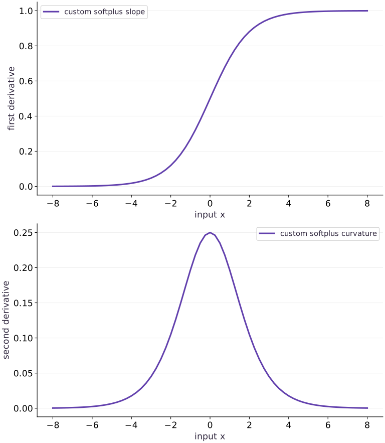
Softplus slope changes from zero to one; its curvature is a symmetric peak of one quarter at zero. — Plot from a recorded CPU computation · JAX 0.9.2 · 1 CPU device

Read the figure

The upper panel plots the first derivative of the custom softplus against its scalar input. It rises smoothly from near zero to near one and passes through $0.5$ at zero. This is sensitivity, not the softplus value itself.

The lower panel plots the second derivative on the same input range. It reaches $0.25$ at zero and falls to about $0.01766$ at both $-4$ and $4$ . The curvature is symmetric even though the first derivative is not.

Connect it to the computation

The plotted values come from differentiating the registered custom rule, including differentiating it twice. Independent sigmoid and sigmoid-times-one-minus-sigmoid formulas check the numerical values at named points. The high-curvature central region is useful for detecting a wrong coefficient.

The separate extreme-input test reaches magnitude one thousand, beyond this display, to check overflow behavior. A smooth curve here is distinct from correctness in every transform or dtype; the VJP interface-boundary experiment and changed-size practice test other parts of the contract.

Open full-size figure Download data and provenance

The notebook contains the data experiment, plotting code, and recorded figure output. Rerun it to test your changes.

Where to put & run this code: Work in phases/14-internals/03-custom-derivative-rules/code/main.py (or downloaded exercises/internals-03.py / exercises/internals-03.ipynb) and execute from the repository root with python3 phases/14-internals/03-custom-derivative-rules/code/main.py.

1 Write stable primal functions and exact derivative contracts

Create main.py for the first block, then append subsequent blocks in order using your course CPU environment.

main.py · append build step 1

# Step 1 — Write stable primal functions and exact derivative contracts: The JVP rule returns primal and tangent; the VJP forward rule...
import jax
# Update state in place with the new values.
jax.config.update("jax_enable_x64", True)
import jax.numpy as jnp
import numpy as np

# Register custom derivative rule on `stable_softplus(x)`:
@jax.custom_jvp
def stable_softplus(x):
    return jnp.logaddexp(0.0,x)

@stable_softplus.defjvp
def softplus_jvp(primals,tangents):
    x,=primals
    dx,=tangents
    return stable_softplus(x),jax.nn.sigmoid(x)*dx

# Register custom derivative rule on `stable_logsumexp(x)`:
@jax.custom_vjp
def stable_logsumexp(x):
    return jax.scipy.special.logsumexp(x)

def logsumexp_fwd(x):
    # Evaluate numerically stable log-space cross-entropy/likelihood (`value`).
    value=stable_logsumexp(x)
    # Apply nonlinear activation or probability normalization to compute `weights`.
    weights=jax.nn.softmax(x)
    return value,weights

def logsumexp_bwd(weights,cotangent):
    return (cotangent*weights,)

# Execute `stable_logsumexp.defvjp(logsumexp_fwd,logsumexp_bwd)`.
stable_logsumexp.defvjp(logsumexp_fwd,logsumexp_bwd)

Code building blocks in this step

config.update(...) — Call config.update with your updated parameters or inputs from this lesson's workspace.
stable_softplus(...) — Call stable_softplus with your updated parameters or inputs from this lesson's workspace.

The JVP rule returns primal and tangent; the VJP forward rule returns primal and residual, and its backward rule returns one cotangent per original input. Both preserve linearity in the directional seed.

2 Check first and second derivatives independently

Create main.py for the first block, then append subsequent blocks in order using your course CPU environment.

main.py · append build step 2

# Step 2 — Check first and second derivatives independently: An exact first derivative can still hide mistakes in a...
points=jnp.array([-4.,0.,3.])
# Vectorize across the batch dimension with `jax.vmap` (`values`).
values=jax.vmap(stable_softplus)(points)
# Differentiate the objective to obtain `first` via automatic differentiation.
first=jax.vmap(jax.grad(stable_softplus))(points)
# Differentiate the objective to obtain `second` via automatic differentiation.
second=jax.vmap(jax.grad(jax.grad(stable_softplus)))(points)
# Convert `reference_first` to a host NumPy array for inspection or verification.
reference_first=1/(1+np.exp(-np.asarray(points)))
reference_second=reference_first*(1-reference_first)
# Convert `` to a host NumPy array for inspection or verification.
np.testing.assert_allclose(values,np.logaddexp(0,np.asarray(points)),rtol=1e-12)
np.testing.assert_allclose(first,reference_first,rtol=1e-12)
np.testing.assert_allclose(second,reference_second,rtol=1e-12)
x=jnp.array([-0.8,0.4,1.1])
# Convert `weights` to a host NumPy array for inspection or verification.
# Accumulate the next contribution into `weights`.
weights=np.exp(np.asarray(x)-np.max(np.asarray(x)))
weights/=weights.sum()
hessian_reference=np.diag(weights)-np.outer(weights,weights)
# Differentiate the objective to obtain gradients ``.
np.testing.assert_allclose(jax.grad(stable_logsumexp)(x),weights,rtol=1e-12)
# Differentiate the objective to obtain gradients ``.
np.testing.assert_allclose(jax.jacrev(jax.grad(stable_logsumexp))(x),hessian_reference,rtol=1e-12,atol=1e-12)
print("Softplus first/second:",np.asarray(first),np.asarray(second))
print("Logsumexp gradient:",weights)

Code building blocks in this step

jnp.array(values, dtype=...) — Constructs an immutable device-backed JAX array from Python/NumPy values.
x.sum(axis=...) / x.mean(axis=..., keepdims=...) — Reduces values along the named axis (the axis you name is collapsed unless keepdims=True).
jnp.allclose(actual, expected, rtol=..., atol=...) — Checks that two arrays match elementwise within floating-point tolerance.
jax.grad(loss_fn)(params, ...) — Transforms a scalar-output function into a function returning the gradient PyTree with the same structure as params.

An exact first derivative can still hide mistakes in a higher-order rule. The softplus curvature and logsumexp Hessian are independently derived here.

3 Exercise extremes and seed linearity

Create main.py for the first block, then append subsequent blocks in order using your course CPU environment.

main.py · append build step 3

# Step 3 — Exercise extremes and seed linearity: Numerical stability must hold in both the primal and derivative path.
extremes=jnp.array([-1000.,0.,1000.])
# Vectorize across the batch dimension with `jax.vmap` (`extreme_values`).
extreme_values=jax.vmap(stable_softplus)(extremes)
# Differentiate the objective to obtain `extreme_gradients` via automatic differentiation.
extreme_gradients=jax.vmap(jax.grad(stable_softplus))(extremes)
# Confirm that all computed values remain finite (no NaN or Inf).
assert np.isfinite(extreme_values).all() and np.isfinite(extreme_gradients).all()
np.testing.assert_allclose(extreme_values,[0.,np.log(2.),1000.],atol=1e-12)
# Enter `np.errstate(over='ignore')` context block:
with np.errstate(over='ignore'):
    # Convert `naive` to a host NumPy array for inspection or verification.
    naive=np.log1p(np.exp(np.asarray(extremes)))
# Confirm that all computed values remain finite (no NaN or Inf).
assert not np.isfinite(naive[-1])
# Compute exact directional derivative / Jacobian / Hessian (`(_, pullback)`).
_,pullback=jax.vjp(stable_logsumexp,x)
np.testing.assert_allclose(pullback(2.0-0.3)[0],2*pullback(1.0)[0]-pullback(0.3)[0],rtol=1e-12)
print("Stable extreme values:",np.asarray(extreme_values),"naive positive extreme:",naive[-1])

Code building blocks in this step

jnp.array(values, dtype=...) — Constructs an immutable device-backed JAX array from Python/NumPy values.
jnp.allclose(actual, expected, rtol=..., atol=...) — Checks that two arrays match elementwise within floating-point tolerance.
jnp.isfinite(x) — Returns a boolean mask verifying that no element is NaN or Inf.
jax.grad(loss_fn)(params, ...) — Transforms a scalar-output function into a function returning the gradient PyTree with the same structure as params.

Numerical stability must hold in both the primal and derivative path. Backward seed linearity is a contract of a true pullback, not an optional aesthetic property.

View the cumulative build in main.py

These blocks append in order to the same file.

main.py · cumulative Python build

# Step 1 — Write stable primal functions and exact derivative contracts: The JVP rule returns primal and tangent; the VJP forward rule...
import jax
# Update state in place with the new values.
jax.config.update("jax_enable_x64", True)
import jax.numpy as jnp
import numpy as np

# Register custom derivative rule on `stable_softplus(x)`:
@jax.custom_jvp
def stable_softplus(x):
    return jnp.logaddexp(0.0,x)

@stable_softplus.defjvp
def softplus_jvp(primals,tangents):
    x,=primals
    dx,=tangents
    return stable_softplus(x),jax.nn.sigmoid(x)*dx

# Register custom derivative rule on `stable_logsumexp(x)`:
@jax.custom_vjp
def stable_logsumexp(x):
    return jax.scipy.special.logsumexp(x)

def logsumexp_fwd(x):
    # Evaluate numerically stable log-space cross-entropy/likelihood (`value`).
    value=stable_logsumexp(x)
    # Apply nonlinear activation or probability normalization to compute `weights`.
    weights=jax.nn.softmax(x)
    return value,weights

def logsumexp_bwd(weights,cotangent):
    return (cotangent*weights,)

# Execute `stable_logsumexp.defvjp(logsumexp_fwd,logsumexp_bwd)`.
stable_logsumexp.defvjp(logsumexp_fwd,logsumexp_bwd)

# Step 2 — Check first and second derivatives independently: An exact first derivative can still hide mistakes in a...
points=jnp.array([-4.,0.,3.])
# Vectorize across the batch dimension with `jax.vmap` (`values`).
values=jax.vmap(stable_softplus)(points)
# Differentiate the objective to obtain `first` via automatic differentiation.
first=jax.vmap(jax.grad(stable_softplus))(points)
# Differentiate the objective to obtain `second` via automatic differentiation.
second=jax.vmap(jax.grad(jax.grad(stable_softplus)))(points)
# Convert `reference_first` to a host NumPy array for inspection or verification.
reference_first=1/(1+np.exp(-np.asarray(points)))
reference_second=reference_first*(1-reference_first)
# Convert `` to a host NumPy array for inspection or verification.
np.testing.assert_allclose(values,np.logaddexp(0,np.asarray(points)),rtol=1e-12)
np.testing.assert_allclose(first,reference_first,rtol=1e-12)
np.testing.assert_allclose(second,reference_second,rtol=1e-12)
x=jnp.array([-0.8,0.4,1.1])
# Convert `weights` to a host NumPy array for inspection or verification.
# Accumulate the next contribution into `weights`.
weights=np.exp(np.asarray(x)-np.max(np.asarray(x)))
weights/=weights.sum()
hessian_reference=np.diag(weights)-np.outer(weights,weights)
# Differentiate the objective to obtain gradients ``.
np.testing.assert_allclose(jax.grad(stable_logsumexp)(x),weights,rtol=1e-12)
# Differentiate the objective to obtain gradients ``.
np.testing.assert_allclose(jax.jacrev(jax.grad(stable_logsumexp))(x),hessian_reference,rtol=1e-12,atol=1e-12)
print("Softplus first/second:",np.asarray(first),np.asarray(second))
print("Logsumexp gradient:",weights)

# Step 3 — Exercise extremes and seed linearity: Numerical stability must hold in both the primal and derivative path.
extremes=jnp.array([-1000.,0.,1000.])
# Vectorize across the batch dimension with `jax.vmap` (`extreme_values`).
extreme_values=jax.vmap(stable_softplus)(extremes)
# Differentiate the objective to obtain `extreme_gradients` via automatic differentiation.
extreme_gradients=jax.vmap(jax.grad(stable_softplus))(extremes)
# Confirm that all computed values remain finite (no NaN or Inf).
assert np.isfinite(extreme_values).all() and np.isfinite(extreme_gradients).all()
np.testing.assert_allclose(extreme_values,[0.,np.log(2.),1000.],atol=1e-12)
# Enter `np.errstate(over='ignore')` context block:
with np.errstate(over='ignore'):
    # Convert `naive` to a host NumPy array for inspection or verification.
    naive=np.log1p(np.exp(np.asarray(extremes)))
# Confirm that all computed values remain finite (no NaN or Inf).
assert not np.isfinite(naive[-1])
# Compute exact directional derivative / Jacobian / Hessian (`(_, pullback)`).
_,pullback=jax.vjp(stable_logsumexp,x)
np.testing.assert_allclose(pullback(2.0-0.3)[0],2*pullback(1.0)[0]-pullback(0.3)[0],rtol=1e-12)
print("Stable extreme values:",np.asarray(extreme_values),"naive positive extreme:",naive[-1])

Run the example

python3 phases/14-internals/03-custom-derivative-rules/code/main.py

About this command

This shortcut uses an activated macOS/Linux course environment in the repository folder. For Windows, use the explicit interpreter command in “Setup help” above. The script includes worked examples and reference solutions.

Inspect the complete assembled example

main.py · complete Python example

# Step 1 — Write stable primal functions and exact derivative contracts: The JVP rule returns primal and tangent; the VJP forward rule...
import jax
# Update state in place with the new values.
jax.config.update("jax_enable_x64", True)
import jax.numpy as jnp
import numpy as np

# Register custom derivative rule on `stable_softplus(x)`:
@jax.custom_jvp
def stable_softplus(x):
    return jnp.logaddexp(0.0,x)

@stable_softplus.defjvp
def softplus_jvp(primals,tangents):
    x,=primals
    dx,=tangents
    return stable_softplus(x),jax.nn.sigmoid(x)*dx

# Register custom derivative rule on `stable_logsumexp(x)`:
@jax.custom_vjp
def stable_logsumexp(x):
    return jax.scipy.special.logsumexp(x)

def logsumexp_fwd(x):
    # Evaluate numerically stable log-space cross-entropy/likelihood (`value`).
    value=stable_logsumexp(x)
    # Apply nonlinear activation or probability normalization to compute `weights`.
    weights=jax.nn.softmax(x)
    return value,weights

def logsumexp_bwd(weights,cotangent):
    return (cotangent*weights,)

# Execute `stable_logsumexp.defvjp(logsumexp_fwd,logsumexp_bwd)`.
stable_logsumexp.defvjp(logsumexp_fwd,logsumexp_bwd)

# Step 2 — Check first and second derivatives independently: An exact first derivative can still hide mistakes in a...
points=jnp.array([-4.,0.,3.])
# Vectorize across the batch dimension with `jax.vmap` (`values`).
values=jax.vmap(stable_softplus)(points)
# Differentiate the objective to obtain `first` via automatic differentiation.
first=jax.vmap(jax.grad(stable_softplus))(points)
# Differentiate the objective to obtain `second` via automatic differentiation.
second=jax.vmap(jax.grad(jax.grad(stable_softplus)))(points)
# Convert `reference_first` to a host NumPy array for inspection or verification.
reference_first=1/(1+np.exp(-np.asarray(points)))
reference_second=reference_first*(1-reference_first)
# Convert `` to a host NumPy array for inspection or verification.
np.testing.assert_allclose(values,np.logaddexp(0,np.asarray(points)),rtol=1e-12)
np.testing.assert_allclose(first,reference_first,rtol=1e-12)
np.testing.assert_allclose(second,reference_second,rtol=1e-12)
x=jnp.array([-0.8,0.4,1.1])
# Convert `weights` to a host NumPy array for inspection or verification.
# Accumulate the next contribution into `weights`.
weights=np.exp(np.asarray(x)-np.max(np.asarray(x)))
weights/=weights.sum()
hessian_reference=np.diag(weights)-np.outer(weights,weights)
# Differentiate the objective to obtain gradients ``.
np.testing.assert_allclose(jax.grad(stable_logsumexp)(x),weights,rtol=1e-12)
# Differentiate the objective to obtain gradients ``.
np.testing.assert_allclose(jax.jacrev(jax.grad(stable_logsumexp))(x),hessian_reference,rtol=1e-12,atol=1e-12)
print("Softplus first/second:",np.asarray(first),np.asarray(second))
print("Logsumexp gradient:",weights)

# Step 3 — Exercise extremes and seed linearity: Numerical stability must hold in both the primal and derivative path.
extremes=jnp.array([-1000.,0.,1000.])
# Vectorize across the batch dimension with `jax.vmap` (`extreme_values`).
extreme_values=jax.vmap(stable_softplus)(extremes)
# Differentiate the objective to obtain `extreme_gradients` via automatic differentiation.
extreme_gradients=jax.vmap(jax.grad(stable_softplus))(extremes)
# Confirm that all computed values remain finite (no NaN or Inf).
assert np.isfinite(extreme_values).all() and np.isfinite(extreme_gradients).all()
np.testing.assert_allclose(extreme_values,[0.,np.log(2.),1000.],atol=1e-12)
# Enter `np.errstate(over='ignore')` context block:
with np.errstate(over='ignore'):
    # Convert `naive` to a host NumPy array for inspection or verification.
    naive=np.log1p(np.exp(np.asarray(extremes)))
# Confirm that all computed values remain finite (no NaN or Inf).
assert not np.isfinite(naive[-1])
# Compute exact directional derivative / Jacobian / Hessian (`(_, pullback)`).
_,pullback=jax.vjp(stable_logsumexp,x)
np.testing.assert_allclose(pullback(2.0-0.3)[0],2*pullback(1.0)[0]-pullback(0.3)[0],rtol=1e-12)
print("Stable extreme values:",np.asarray(extreme_values),"naive positive extreme:",naive[-1])

Expected result: Softplus derivatives at zero are 0.5 and 0.25. Stable values at [-1000, 0, 1000] are [0, log(2), 1000]; the naive positive extreme overflows. The custom reverse Hessian matches diag(p)-p p-transpose.

Recorded reference execution

Reference output captured from executing the complete lesson script (code/main.py) and its assertions in the course CPU environment.

2026-10-20T10:50:14.579922+00:00 · Python 3.14.3 · JAX 0.9.2 · 1 CPU device

Softplus first/second: [0.01798621 0.5        0.95257413] [0.01766271 0.25       0.04517666]
Logsumexp gradient: [0.09085944 0.30166396 0.60747661]
Stable extreme values: [0.00000000e+00 6.93147181e-01 1.00000000e+03] naive positive extreme: inf
Softplus first/second: [0.01798621 0.5        0.95257413] [0.01766271 0.25       0.04517666]
Logsumexp gradient: [0.09085944 0.30166396 0.60747661]
Stable extreme values: [0.00000000e+00 6.93147181e-01 1.00000000e+03] naive positive extreme: inf
Wrong/correct/finite-difference derivative: 0.29934383005622606 0.5986876601124521 0.5986876601138391
Expected custom_vjp forward-mode boundary: can't apply forward-mode autodiff (jvp) to a custom_vjp function.
Ordinary JAX common-shift JVP: 1.0
Changed-size gradient and cotangent scaling verified
Stable shift invariance and zero common-direction curvature verified
Nonlinear seed rule rejected by its contract; repaired JVP is linear
PASS: internals-03

Download execution record · The notebook includes executed cells and figure outputs. Compare your run with these values; timings depend on the machine.

Expose a wrong but linear rule

Expose a wrong but linear rule · Python experiment

# Experiment — Expose a wrong but linear rule: The wrong tangent expression is linear, so transposition can...
# Register custom derivative rule on `wrong_softplus(z)`:
@jax.custom_jvp
def wrong_softplus(z):
    return jnp.logaddexp(0.0,z)
@wrong_softplus.defjvp
def wrong_rule(primals,tangents):
    z,=primals
    dz,=tangents
    return wrong_softplus(z),0.5*jax.nn.sigmoid(z)*dz
probe=0.4
eps=1e-5
finite=(np.logaddexp(0,probe+eps)-np.logaddexp(0,probe-eps))/(2*eps)
# Differentiate the objective to obtain `wrong` via automatic differentiation.
wrong=float(jax.grad(wrong_softplus)(probe))
# Differentiate the objective to obtain `right` via automatic differentiation.
right=float(jax.grad(stable_softplus)(probe))
assert abs(wrong-finite)>0.2
np.testing.assert_allclose(right,finite,rtol=1e-9)
print("Wrong/correct/finite-difference derivative:",wrong,right,finite)

Expected: Wrong derivative approximately 0.29934; correct and finite-difference derivatives approximately 0.59869.

The wrong tangent expression is linear, so transposition can still work. Only an independent mathematical or numerical oracle detects its incorrect coefficient.

Exercise the custom VJP boundary

Exercise the custom VJP boundary · Python experiment

# Experiment — Exercise the custom VJP boundary: Adding the same constant to all logits shifts log-sum-exp by...
rejected=False
# Run the boundary check and catch the expected exception:
try:
    jax.jvp(stable_logsumexp,(x,),(jnp.ones_like(x),))
except TypeError as error:
    rejected=True
    print("Expected custom_vjp forward-mode boundary:",str(error).splitlines()[0])
assert rejected
# Evaluate numerically stable log-space cross-entropy/likelihood (`ordinary`).
ordinary=lambda z:jax.scipy.special.logsumexp(z)
# Compute exact directional derivative / Jacobian / Hessian (`ordinary_direction`).
ordinary_direction=jax.jvp(ordinary,(x,),(jnp.ones_like(x),))[1]
np.testing.assert_allclose(ordinary_direction,1.0,atol=1e-12)
print("Ordinary JAX common-shift JVP:",float(ordinary_direction))

Expected: The custom_vjp direct JVP is rejected; the ordinary function gives directional derivative 1.

Adding the same constant to all logits shifts log-sum-exp by that constant. The mathematical derivative exists; the limitation belongs to the custom_vjp transformation interface.

Hands-On Exercise · Modify & Verify Run in the declared lesson environment

Make it yours

Where to put your code: Append your solution at the bottom of phases/14-internals/03-custom-derivative-rules/code/main.py (or inside the Make it yours cell of exercises/internals-03.ipynb) and run python3 phases/14-internals/03-custom-derivative-rules/code/main.py to verify your prediction before opening the reference solution.

Check the custom log-sum-exp gradient on $(-3,0.2,2,5)$ against an independent stable softmax and central differences along two directions. Keep the output cotangent explicit.

Show a writing guide and starter scaffold

How to write this exercise code: step-by-step recipe & starter scaffold

1. Key functions & syntax to use:

jnp.array(values, dtype=...) — Constructs an immutable device-backed JAX array from Python/NumPy values.
x.sum(axis=...) / x.mean(axis=..., keepdims=...) — Reduces values along the named axis (the axis you name is collapsed unless keepdims=True).
jnp.allclose(actual, expected, rtol=..., atol=...) — Checks that two arrays match elementwise within floating-point tolerance.
jax.grad(loss_fn)(params, ...) — Transforms a scalar-output function into a function returning the gradient PyTree with the same structure as params.

2. Step-by-step implementation plan:

Convert host to a host NumPy array for inspection or verification.
Accumulate the next contribution into p.
Differentiate the objective to obtain actual via automatic differentiation.
Aggregate array values to compute reference.
Convert to a host NumPy array for inspection or verification.

Starter code scaffold · copy into your file & fill in the TODOs

# Exercise solution: Check the custom log-sum-exp gradient on (-3,0.2,2,5) against an...
changed = jnp.array(...)  # TODO: compute changed
# Convert `host` to a host NumPy array for inspection or verification.
# Accumulate the next contribution into `p`.
host = np.asarray(...)  # TODO: compute host
p = np.exp(...)  # TODO: compute p
p/=p.sum()
# Differentiate the objective to obtain `actual` via automatic differentiation.
actual = jax.grad(...)  # TODO: compute actual
np.testing.assert_allclose(actual,p,rtol = ...  # TODO: compute np.testing.assert_allclose(actual,p,rtol
for direction in (np.array([1.,-.5,.2,0.]),np.array([0.,1.,-1.,.3])):
    eps = ...  # TODO: compute eps
    # Aggregate array values to compute `reference`.
    reference = ...  # TODO: compute reference
    fd = ...  # TODO: compute fd
    # Convert `` to a host NumPy array for inspection or verification.
    np.testing.assert_allclose(np.dot(np.asarray(actual),direction),fd,rtol = ...  # TODO: compute np.testing.assert_allclose(np.dot(np.asarray(actual),direction),fd,rtol
np.testing.assert_allclose(jax.vjp(stable_logsumexp,changed)[1](2.5)[0],2.5*p,rtol=1e-12)
print("Changed-size gradient and cotangent scaling verified")

Reveal the reference solution

Reference solution

# Exercise solution: Check the custom log-sum-exp gradient on (-3,0.2,2,5) against an...
changed=jnp.array([-3.,0.2,2.,5.])
# Convert `host` to a host NumPy array for inspection or verification.
# Accumulate the next contribution into `p`.
host=np.asarray(changed)
p=np.exp(host-host.max())
p/=p.sum()
# Differentiate the objective to obtain `actual` via automatic differentiation.
actual=jax.grad(stable_logsumexp)(changed)
np.testing.assert_allclose(actual,p,rtol=1e-12)
for direction in (np.array([1.,-.5,.2,0.]),np.array([0.,1.,-1.,.3])):
    eps=1e-5
    # Aggregate array values to compute `reference`.
    reference=lambda z:np.max(z)+np.log(np.exp(z-np.max(z)).sum())
    fd=(reference(host+eps*direction)-reference(host-eps*direction))/(2*eps)
    # Convert `` to a host NumPy array for inspection or verification.
    np.testing.assert_allclose(np.dot(np.asarray(actual),direction),fd,rtol=1e-8,atol=1e-10)
np.testing.assert_allclose(jax.vjp(stable_logsumexp,changed)[1](2.5)[0],2.5*p,rtol=1e-12)
print("Changed-size gradient and cotangent scaling verified")

Check common-shift invariance of curvature

Practice

Add a common constant of $1000$ to every logit. Verify the value shift, unchanged gradient, and Hessian row sums.

Show a writing guide and starter scaffold

How to write this practice solution: step-by-step recipe & starter scaffold

1. Key functions & syntax to use:

x.sum(axis=...) / x.mean(axis=..., keepdims=...) — Reduces values along the named axis (the axis you name is collapsed unless keepdims=True).
jnp.allclose(actual, expected, rtol=..., atol=...) — Checks that two arrays match elementwise within floating-point tolerance.
jax.grad(loss_fn)(params, ...) — Transforms a scalar-output function into a function returning the gradient PyTree with the same structure as params.
jax.jvp / jax.vjp / jax.jacfwd / jax.hessian — Computes exact forward-mode JVP, reverse-mode VJP, full Jacobians, or second-order curvature.

2. Step-by-step implementation plan:

Differentiate the objective to obtain gradients .
Differentiate the objective to obtain hess via automatic differentiation.

Starter code scaffold · copy into your file & fill in the TODOs

# Check common-shift invariance of curvature (Practice): The common shift leaves probabilities unchanged.
shift = ...  # TODO: compute shift
np.testing.assert_allclose(stable_logsumexp(x+shift)-stable_logsumexp(x),shift,rtol=1e-12)
# Differentiate the objective to obtain gradients ``.
np.testing.assert_allclose(jax.grad(stable_logsumexp)(x+shift),jax.grad(stable_logsumexp)(x),rtol=1e-12)
# Differentiate the objective to obtain `hess` via automatic differentiation.
hess = jax.jacrev(...)  # TODO: compute hess
np.testing.assert_allclose(jnp.sum(hess,axis = ...  # TODO: compute np.testing.assert_allclose(jnp.sum(hess,axis
print("Stable shift invariance and zero common-direction curvature verified")

Show a hint

Use stable references and avoid direct exponentiation of the shifted logits.

Reveal reference solution and reasoning

Check common-shift invariance of curvature · Python solution

# Check common-shift invariance of curvature (Practice): The common shift leaves probabilities unchanged.
shift=1000.0
np.testing.assert_allclose(stable_logsumexp(x+shift)-stable_logsumexp(x),shift,rtol=1e-12)
# Differentiate the objective to obtain gradients ``.
np.testing.assert_allclose(jax.grad(stable_logsumexp)(x+shift),jax.grad(stable_logsumexp)(x),rtol=1e-12)
# Differentiate the objective to obtain `hess` via automatic differentiation.
hess=jax.jacrev(jax.grad(stable_logsumexp))(x+shift)
np.testing.assert_allclose(jnp.sum(hess,axis=1),0.,atol=1e-12)
print("Stable shift invariance and zero common-direction curvature verified")

The common shift leaves probabilities unchanged. Zero curvature in that direction is a structural identity, not a numerical accident.

Audit a nonlinear seed rule before registering it

Challenge

A proposed JVP returns $\sigma(x)\dot{x}^2$ . Show explicitly why it cannot be the derivative map, then repair it and test a mixed linear combination.

Show a writing guide and starter scaffold

How to write this practice solution: step-by-step recipe & starter scaffold

1. Key functions & syntax to use:

jnp.array(values, dtype=...) — Constructs an immutable device-backed JAX array from Python/NumPy values.
jnp.allclose(actual, expected, rtol=..., atol=...) — Checks that two arrays match elementwise within floating-point tolerance.
jax.jvp / jax.vjp / jax.jacfwd / jax.hessian — Computes exact forward-mode JVP, reverse-mode VJP, full Jacobians, or second-order curvature.

2. Step-by-step implementation plan:

Compute exact directional derivative / Jacobian / Hessian (good).

Starter code scaffold · copy into your file & fill in the TODOs

# Audit a nonlinear seed rule before registering it (Challenge): Linearity follows from the definition of a derivative at a...
coefficient = float(...)  # TODO: compute coefficient
bad = ...  # TODO: compute bad
assert not np.isclose(bad(2.0),2*bad(1.0))  # TODO: complete assertion check
# Compute exact directional derivative / Jacobian / Hessian (`good`).
good = ...  # TODO: compute good
np.testing.assert_allclose(good(2*.7-.3),2*good(.7)-good(.3),rtol=1e-12)
print("Nonlinear seed rule rejected by its contract; repaired JVP is linear")

Show a hint

At fixed x, compare the response to twice a tangent with twice the response.

Reveal reference solution and reasoning

Audit a nonlinear seed rule before registering it · Python solution

# Audit a nonlinear seed rule before registering it (Challenge): Linearity follows from the definition of a derivative at a...
coefficient=float(jax.nn.sigmoid(0.4))
bad=lambda tangent:coefficient*tangent*tangent
assert not np.isclose(bad(2.0),2*bad(1.0))
# Compute exact directional derivative / Jacobian / Hessian (`good`).
good=lambda tangent:jax.jvp(stable_softplus,(jnp.array(0.4),),(jnp.array(tangent),))[1]
np.testing.assert_allclose(good(2*.7-.3),2*good(.7)-good(.3),rtol=1e-12)
print("Nonlinear seed rule rejected by its contract; repaired JVP is linear")

Linearity follows from the definition of a derivative at a fixed primal point. API acceptance is not a substitute for this mathematical check.

Diagnose the result

If first derivatives pass but second derivatives fail, inspect whether residuals or derivative coefficients have been detached. If extreme values are nonfinite, inspect both primal and derivative expressions. If a custom VJP direct JVP fails, treat that as an interface boundary. If a plausible custom gradient differs from finite differences, do not relabel it exact without a valid derivation.

Carry forward

Keep the primal stable before customizing its derivative
A custom JVP must remain linear in its tangent
Choose residuals for a custom reverse pass
Higher-order behavior is part of the promise
Custom reverse mode has a transformation boundary
An intentionally different gradient needs a different claim

Keep your evidence

Download evidence template

Stable extreme inputs, analytic slopes/Hessians, seed linearity, independent finite differences and a deliberately wrong-rule diagnosis. Keep the environment, observed outputs and your explanation of the figure.

Save your modified code, its output, and an explanation of your prediction. Checkpoint answers and exercise evidence are tracked separately.

Saved in this browser. Export or back up your portfolio anytime in My learning.

Save work for this lesson

Verified on local CPU. Stage to a Cloud TPU VM via Cloud TPU setup to record accelerator execution receipts (TODO: add automated Cloud TPU CI execution receipts).

Custom derivative rules

What you will be able to do

The problem

The idea

A custom rule is a mathematical contract

Keep the primal stable before customizing its derivative

A custom JVP must remain linear in its tangent

Choose residuals for a custom reverse pass

Higher-order behavior is part of the promise

Custom reverse mode has a transformation boundary

An intentionally different gradient needs a different claim

A stable custom rule preserves both slope and curvature

Read the figure

Connect it to the computation

1 Write stable primal functions and exact derivative contracts

2 Check first and second derivatives independently

3 Exercise extremes and seed linearity

Run the example

Recorded reference execution

Expose a wrong but linear rule

Exercise the custom VJP boundary

Make it yours

Check common-shift invariance of curvature

Audit a nonlinear seed rule before registering it

Check your understanding

Diagnose the result

Carry forward

Keep your evidence

Primary references