 JAX Pathways
Phase 05 / Neural network training
Build a tiny multilayer perceptron
Revision v0.7.0 · Updated since your last visit. Review the changes; your progress is saved.
Lesson · about 85 minutes · CPU practice
Implement a small model with explicit parameters before adding a model library.
Phase study guide: preparation, milestones and project evidence
Before you start
Before this: Math & optimization
Hardware: CPU
Setup help: Python, notebook, or Cloud TPU VM
Use the tested CPU packages (the recorded environment uses Python 3.14.3). Other Python versions and accelerator environments require separate checks. The optional Cloud TPU specialization explains the target-specific execution boundaries. Logical CPU devices practice partitioning; they do not simulate TPU performance.
Download the repository ZIP or use your existing checkout. Extract it and open a terminal in the folder containing requirements-cpu.txt. The beginner ZIP is separate; these lessons use the full repository folder.
python3 -m venv .venv
source .venv/bin/activate
python -m pip install -r requirements-cpu.txtpy -3 -m venv .venv
.\.venv\Scripts\python.exe -m pip install -r requirements-cpu.txtAfter activation, run the complete worked example from that same folder:
python phases/05-networks/01-build-a-tiny-multilayer-perceptron/code/main.py.\.venv\Scripts\python.exe phases/05-networks/01-build-a-tiny-multilayer-perceptron/code/main.pyFor an incremental build, create main.py in your own practice folder, append each build block in order, and run python main.py with this environment active. Keep that file separate from the downloaded reference solution.
Download this lesson’s notebook. Open it with a Python kernel using the course environment. Run cells from the top after restarting the kernel; experiments depend on earlier definitions.
For local Jupyter, first install the course requirements using the Local Python steps, then use your environment’s Python to start Jupyter:
python -m pip install jupyterlab
python -m jupyter lab.\.venv\Scripts\python.exe -m pip install jupyterlab
.\.venv\Scripts\python.exe -m jupyter labSelect the downloaded networks-01.ipynb file in JupyterLab. The notebook contains reference solutions; make your prediction and attempt each practice task before opening them. Restart the kernel before changing logical device setup.
The worked reference for this lesson is CPU-validated. Some references explicitly configure logical CPU devices; setting JAX_PLATFORMS does not adapt them to a TPU. Follow the execution matrix and reviewed multi-host example before attempting a target run.
For accelerator preparation, study TPU setup, observed runtime receipts, checkpointed jobs and precision and retained traces. These target paths remain unqualified on physical TPU hardware until an actual receipt is recorded. Cloud provisioning is optional for CPU learning.
Check: Loss falls below and nearby held-out accuracy is at least . Exact initialization and losses may vary across backend/version.
Revisit the guided CPU setup · Open 19: TPU Setup. Package instructions are CPU instructions; Windows and accelerator environments need their own validation.
What you will be able to do
- Trace the shapes from observations to logits
- Explain why the hidden activation matters
- Use stable binary cross-entropy
- Separate learning from held-out measurement
The problem
Four points can give us a useful puzzle: how do we separate the two diagonal pairs in XOR? A single straight line cannot do it. We’ll add a small hidden layer and a nonlinear activation, check the shapes, and train a classifier. Then we’ll test nearby points to see what it has learned beyond the four training examples.
The idea
A multilayer perceptron combines learned linear maps with nonlinear activations. The hidden layer builds features that the output layer can combine. The activation lets the composition represent boundaries that a single linear map cannot.
Why hidden layers need nonlinear operations
XOR gives the same label to opposite corners of a square. One straight separating line cannot isolate both opposite corners from the other two. Hidden units can form intermediate regions that an output layer combines.
Remove every nonlinear activation and the weight matrices simply multiply into one linear map. More matrices alone do not solve this geometry. Biases change offsets but do not remove the limitation.
Read the decision field both at and between the training points. The four observed labels constrain only a tiny part of the plane. A smooth-looking boundary is still an extrapolation. Connect each layer's actual width to the feature vector it produces before interpreting that extrapolation.
Trace the shapes from observations to logits
Each row is one observation with two features. The first weight matrix has shape , so a batch becomes . A bias vector broadcasts across rows; it does not create eight observations. tanh changes values without changing shape. The second matrix produces one logit per row. Squeeze only the final axis to produce , preserving the batch dimension even when is one. A logit is an unrestricted real score; a positive logit predicts class one when the decision threshold is probability .
(B, 2) → affine → (B, 8) → tanh → (B, 8) → affine → (B, 1) → (B,)Explain why the hidden activation matters
XOR assigns matching signs to class zero and opposite signs to class one. A single line cannot place both diagonal pairs on opposite sides. Two affine layers without an activation still collapse to one affine map: ( W1 + b1) W2 + b2. More parameters alone therefore do not solve this obstacle. tanh introduces curved intermediate features that can support a nonlinear boundary. Eight hidden units are deliberately small enough to inspect. They are not a principled best width, and successful training at one seed does not guarantee every initialization will converge.
Use stable binary cross-entropy
Do not calculate by separately taking the sigmoid and logarithm. At large negative scores the probability may round to zero. The stable scalar loss is . Average these losses over the batch so duplicating every row does not double the objective. Labels are zero or one, logits and labels both have shape , and gradients are taken with respect to the parameter tree. The derivative with respect to each score is , divided by batch size. We verify the implementation independently with NumPy and verify a zero-parameter example against .
Separate learning from held-out measurement
The four XOR corners are the complete training set. Held-out points are perturbed versions of those corners, generated from a separate fixed seed. Their labels follow the original sign rule. They check nearby transfer rather than merely memorizing four exact inputs. They do not test arbitrary extrapolation across the plane; this small fixture is especially easy. Record initial and final loss, the seed, hidden width, learning rate, update count, and held-out accuracy. Keep evaluation outside the update loop and do not select a hyperparameter by repeatedly inspecting the held-out answers.
Read the classification loss one example at a time
The logit is the model’s raw score; the label is either or . A positive logit favors class . When , the sigmoid probability is one half, so either label gives a loss of . That is a useful sanity check. In code, logaddexp evaluates the softplus term stably instead of separately computing an exponential and logarithm.
A tiny MLP separates the XOR regions
Predict before looking: Can a single straight boundary separate these labels?
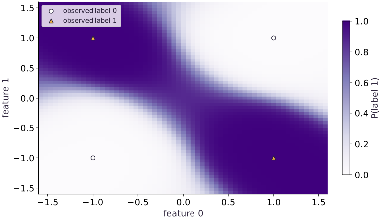
Read the figure
The axes are the two input features. Background color shows the model’s predicted probability of label : dark purple is near , and the pale regions are near . The markers give observed labels independently of that background: triangles are label , circles are label .
The triangles at and sit in dark regions. The circles at and sit in pale regions. Thus the learned pattern assigns label to opposite-sign corners and label to same-sign corners, matching XOR.
Connect it to the computation
A single straight boundary cannot separate these alternating corners. The hidden nonlinear layer allows the model to bend the boundary and create separated regions for the same class. The transition band between light and dark marks inputs where the predicted probability changes rapidly.
Most colored locations are grid queries, not additional labeled observations. Their colors show how this trained model extends its predictions between and beyond the examples. A dark region alone is separate from calibrated confidence or accuracy there; those claims need appropriate held-out data.
Open full-size figureDownload data and provenance
The notebook contains the data experiment, plotting code, and recorded figure output. Rerun it to test your changes.
Where to put & run this code: Work in phases/05-networks/01-build-a-tiny-multilayer-perceptron/code/main.py (or downloaded exercises/networks-01.py / exercises/networks-01.ipynb) and execute from the repository root with python3 phases/05-networks/01-build-a-tiny-multilayer-perceptron/code/main.py.
1 Define the fixture and parameter tree
Create main.py and copy this block. Before running, write the four XOR labels and the expected shape of each parameter.
# Step 1 — 1. Define the fixture and parameter tree: The parameter count is 16+8+8+1=33.
import jax
import jax.numpy as jnp
import numpy as np
import optax
x = jnp.array([[-1.,-1.],[-1.,1.],[1.,-1.],[1.,1.]])
y = jnp.array([0.,1.,1.,0.])
# Create or split explicit PRNG key(s) (`(k1, k2)`) for reproducible randomness.
k1, k2 = jax.random.split(jax.random.key(0))
# Sample deterministic random values into `params` using an explicit PRNG key.
params = {'w1':jax.random.normal(k1,(2,8))*.4, 'b1':jnp.zeros(8),
          'w2':jax.random.normal(k2,(8,1))*.4, 'b2':jnp.zeros(1)}
assert sum(a.size for a in jax.tree.leaves(params)) == 33
Code building blocks in this step
jnp.array(values, dtype=...)— Constructs an immutable device-backed JAX array from Python/NumPy values.jnp.zeros / jnp.ones(shape, dtype=...)— Allocates a tensor of the givenshapeinitialized with constants.jax.random.PRNGKey(seed) & jax.random.split(key)— Manages explicit, stateless PRNG keys—always split a key before passing subkeys into independent random draws.
The parameter count is . Independent keys initialize the two layers; biases start at zero.
2 Write prediction and verify the loss
Append these functions. The NumPy reference has no autodiff or optimizer and tests the objective itself.
# Step 2 — 2. Write prediction and verify the loss: The zero-score baseline is about 0.693147.
def logits(p, batch):
    return (jnp.tanh(batch@p['w1']+p['b1'])@p['w2']+p['b2']).squeeze(-1)
def loss(p, batch, labels):
    return jnp.mean(optax.sigmoid_binary_cross_entropy(logits(p,batch),labels))
# Convert `scores` to a host NumPy array for inspection or verification.
scores = np.asarray(logits(params,x))
# Aggregate array values to compute `expected`.
expected = np.mean(np.logaddexp(0.,scores)-np.asarray(y)*scores)
np.testing.assert_allclose(loss(params,x,y), expected, rtol=1e-6)
# Transform every leaf of the parameter PyTree (`zeros`).
zeros = jax.tree.map(jnp.zeros_like, params)
np.testing.assert_allclose(loss(zeros,x,y),np.log(2.),rtol=1e-6)
# Check tensor shape invariant: `logits(params,jnp.ones((1,2))).shape == (1,)`
assert logits(params,jnp.ones((1,2))).shape == (1,)
Code building blocks in this step
jnp.zeros / jnp.ones(shape, dtype=...)— Allocates a tensor of the givenshapeinitialized with constants.x.sum(axis=...) / x.mean(axis=..., keepdims=...)— Reduces values along the namedaxis(the axis you name is collapsed unlesskeepdims=True).jnp.allclose(actual, expected, rtol=..., atol=...)— Checks that two arrays match elementwise within floating-point tolerance.jax.tree.map(lambda p, g: ..., params, grads)— Applies a function leaf-by-leaf across matching PyTrees (such as updating every parameter tensor with its gradient).
The zero-score baseline is about . A loss below it alone does not prove held-out skill.
3 Train and evaluate untouched points
Append the compiled step and loop. Prediction: can the nonlinear model beat chance on points near each training corner?
# Step 3 — 3. Train and evaluate untouched points: The independent held-out seed changes input coordinates.
# Configure or step the Optax optimizer state (`tx`).
tx = optax.adam(.03)
state = tx.init(params)
# Define and JIT-compile `step(p, s)` so XLA traces and fuses the operations:
@jax.jit
def step(p,s):
    # Differentiate the objective to obtain `(value, grads)` via automatic differentiation.
    value,grads = jax.value_and_grad(loss)(p,x,y)
    updates,s = tx.update(grads,s,p)
    return optax.apply_updates(p,updates),s,value
initial = float(loss(params,x,y))
for _ in range(200): params,state,_ = step(params,state)
# Draw pseudorandom samples for `rng` using the explicit RNG state.
rng = np.random.default_rng(12)
# Convert `held_x` to a host NumPy array for inspection or verification.
held_x = np.repeat(np.asarray(x),8,axis=0)+rng.normal(0,.12,(32,2))
held_y = (held_x[:,0]*held_x[:,1]<0).astype(np.float32)
held_scores = np.asarray(logits(params,jnp.array(held_x)))
# Aggregate array values to compute `accuracy`.
accuracy = np.mean((held_scores>0)==held_y)
final = float(loss(params,x,y))
assert final < .03 and accuracy >= .95
print('Training loss:', initial, '->', final, 'held-out accuracy:', accuracy)
Code building blocks in this step
jnp.array(values, dtype=...)— Constructs an immutable device-backed JAX array from Python/NumPy values.x.sum(axis=...) / x.mean(axis=..., keepdims=...)— Reduces values along the namedaxis(the axis you name is collapsed unlesskeepdims=True).jax.value_and_grad(loss_fn)(params, ...)— Evaluates both the scalar loss and its gradient PyTree(loss_val, grads)in a single forward+backward pass.jax.jit(fn) / @jax.jit— Tracesfnwith abstract shapes and compiles a fused XLA executable cached by input shape and dtype.
The independent held-out seed changes input coordinates. Passing this check establishes behavior on this fixture only.
View the cumulative build in main.py
These blocks append in order to the same file.
# Step 1 — 1. Define the fixture and parameter tree: The parameter count is 16+8+8+1=33.
import jax
import jax.numpy as jnp
import numpy as np
import optax
x = jnp.array([[-1.,-1.],[-1.,1.],[1.,-1.],[1.,1.]])
y = jnp.array([0.,1.,1.,0.])
# Create or split explicit PRNG key(s) (`(k1, k2)`) for reproducible randomness.
k1, k2 = jax.random.split(jax.random.key(0))
# Sample deterministic random values into `params` using an explicit PRNG key.
params = {'w1':jax.random.normal(k1,(2,8))*.4, 'b1':jnp.zeros(8),
          'w2':jax.random.normal(k2,(8,1))*.4, 'b2':jnp.zeros(1)}
assert sum(a.size for a in jax.tree.leaves(params)) == 33

# Step 2 — 2. Write prediction and verify the loss: The zero-score baseline is about 0.693147.
def logits(p, batch):
    return (jnp.tanh(batch@p['w1']+p['b1'])@p['w2']+p['b2']).squeeze(-1)
def loss(p, batch, labels):
    return jnp.mean(optax.sigmoid_binary_cross_entropy(logits(p,batch),labels))
# Convert `scores` to a host NumPy array for inspection or verification.
scores = np.asarray(logits(params,x))
# Aggregate array values to compute `expected`.
expected = np.mean(np.logaddexp(0.,scores)-np.asarray(y)*scores)
np.testing.assert_allclose(loss(params,x,y), expected, rtol=1e-6)
# Transform every leaf of the parameter PyTree (`zeros`).
zeros = jax.tree.map(jnp.zeros_like, params)
np.testing.assert_allclose(loss(zeros,x,y),np.log(2.),rtol=1e-6)
# Check tensor shape invariant: `logits(params,jnp.ones((1,2))).shape == (1,)`
assert logits(params,jnp.ones((1,2))).shape == (1,)

# Step 3 — 3. Train and evaluate untouched points: The independent held-out seed changes input coordinates.
# Configure or step the Optax optimizer state (`tx`).
tx = optax.adam(.03)
state = tx.init(params)
# Define and JIT-compile `step(p, s)` so XLA traces and fuses the operations:
@jax.jit
def step(p,s):
    # Differentiate the objective to obtain `(value, grads)` via automatic differentiation.
    value,grads = jax.value_and_grad(loss)(p,x,y)
    updates,s = tx.update(grads,s,p)
    return optax.apply_updates(p,updates),s,value
initial = float(loss(params,x,y))
for _ in range(200): params,state,_ = step(params,state)
# Draw pseudorandom samples for `rng` using the explicit RNG state.
rng = np.random.default_rng(12)
# Convert `held_x` to a host NumPy array for inspection or verification.
held_x = np.repeat(np.asarray(x),8,axis=0)+rng.normal(0,.12,(32,2))
held_y = (held_x[:,0]*held_x[:,1]<0).astype(np.float32)
held_scores = np.asarray(logits(params,jnp.array(held_x)))
# Aggregate array values to compute `accuracy`.
accuracy = np.mean((held_scores>0)==held_y)
final = float(loss(params,x,y))
assert final < .03 and accuracy >= .95
print('Training loss:', initial, '->', final, 'held-out accuracy:', accuracy)
Run the example
python3 phases/05-networks/01-build-a-tiny-multilayer-perceptron/code/main.pyAbout this command
This shortcut uses an activated macOS/Linux course environment in the repository folder. For Windows, use the explicit interpreter command in “Setup help” above. The script includes worked examples and reference solutions.
Inspect the complete assembled example
# Step 1 — 1. Define the fixture and parameter tree: The parameter count is 16+8+8+1=33.
import jax
import jax.numpy as jnp
import numpy as np
import optax
x = jnp.array([[-1.,-1.],[-1.,1.],[1.,-1.],[1.,1.]])
y = jnp.array([0.,1.,1.,0.])
# Create or split explicit PRNG key(s) (`(k1, k2)`) for reproducible randomness.
k1, k2 = jax.random.split(jax.random.key(0))
# Sample deterministic random values into `params` using an explicit PRNG key.
params = {'w1':jax.random.normal(k1,(2,8))*.4, 'b1':jnp.zeros(8),
          'w2':jax.random.normal(k2,(8,1))*.4, 'b2':jnp.zeros(1)}
assert sum(a.size for a in jax.tree.leaves(params)) == 33

# Step 2 — 2. Write prediction and verify the loss: The zero-score baseline is about 0.693147.
def logits(p, batch):
    return (jnp.tanh(batch@p['w1']+p['b1'])@p['w2']+p['b2']).squeeze(-1)
def loss(p, batch, labels):
    return jnp.mean(optax.sigmoid_binary_cross_entropy(logits(p,batch),labels))
# Convert `scores` to a host NumPy array for inspection or verification.
scores = np.asarray(logits(params,x))
# Aggregate array values to compute `expected`.
expected = np.mean(np.logaddexp(0.,scores)-np.asarray(y)*scores)
np.testing.assert_allclose(loss(params,x,y), expected, rtol=1e-6)
# Transform every leaf of the parameter PyTree (`zeros`).
zeros = jax.tree.map(jnp.zeros_like, params)
np.testing.assert_allclose(loss(zeros,x,y),np.log(2.),rtol=1e-6)
# Check tensor shape invariant: `logits(params,jnp.ones((1,2))).shape == (1,)`
assert logits(params,jnp.ones((1,2))).shape == (1,)

# Step 3 — 3. Train and evaluate untouched points: The independent held-out seed changes input coordinates.
# Configure or step the Optax optimizer state (`tx`).
tx = optax.adam(.03)
state = tx.init(params)
# Define and JIT-compile `step(p, s)` so XLA traces and fuses the operations:
@jax.jit
def step(p,s):
    # Differentiate the objective to obtain `(value, grads)` via automatic differentiation.
    value,grads = jax.value_and_grad(loss)(p,x,y)
    updates,s = tx.update(grads,s,p)
    return optax.apply_updates(p,updates),s,value
initial = float(loss(params,x,y))
for _ in range(200): params,state,_ = step(params,state)
# Draw pseudorandom samples for `rng` using the explicit RNG state.
rng = np.random.default_rng(12)
# Convert `held_x` to a host NumPy array for inspection or verification.
held_x = np.repeat(np.asarray(x),8,axis=0)+rng.normal(0,.12,(32,2))
held_y = (held_x[:,0]*held_x[:,1]<0).astype(np.float32)
held_scores = np.asarray(logits(params,jnp.array(held_x)))
# Aggregate array values to compute `accuracy`.
accuracy = np.mean((held_scores>0)==held_y)
final = float(loss(params,x,y))
assert final < .03 and accuracy >= .95
print('Training loss:', initial, '->', final, 'held-out accuracy:', accuracy)
Expected result: Loss falls below and nearby held-out accuracy is at least . Exact initialization and losses may vary across backend/version.
Recorded reference execution
Reference output captured from executing the complete lesson script (code/main.py) and its assertions in the course CPU environment.
Training loss: 0.7047799825668335 -> 0.0015878621488809586 held-out accuracy: 1.0
Training loss: 0.7047799825668335 -> 0.0015878621488809586 held-out accuracy: 1.0
Consistent hidden permutation preserves logits; one-sided permutation changes them.
PASS: networks-01
Download execution record · The notebook includes executed cells and figure outputs. Compare your run with these values; timings depend on the machine.
Duplication preserves a mean objective
# Experiment — Duplication preserves a mean objective: Averaging normalizes repeated identical data.
repeated_x=jnp.repeat(x,3,axis=0)
repeated_y=jnp.repeat(y,3)
np.testing.assert_allclose(loss(params,repeated_x,repeated_y),loss(params,x,y),rtol=1e-5)
# Differentiate the objective to obtain `original_g` via automatic differentiation.
original_g=jax.grad(loss)(params,x,y)
repeated_g=jax.grad(loss)(params,repeated_x,repeated_y)
for a,b in zip(jax.tree.leaves(original_g),jax.tree.leaves(repeated_g)):
    np.testing.assert_allclose(a,b,rtol=1e-4,atol=1e-7)
Expected: The losses and corresponding gradient leaves agree within tolerance.
Averaging normalizes repeated identical data. Summing would change the learning-rate interpretation.
An affine stack stays affine
# Experiment — An affine stack stays affine: This exact affine identity explains why removing the...
def affine_stack(batch):return (batch@params['w1']+params['b1'])@params['w2']+params['b2']
midpoint=jnp.array([[.2,-.3]])
delta=jnp.array([[.4,.1]])
# Combine or mask array elements to form ``.
np.testing.assert_allclose(affine_stack(midpoint),.5*(affine_stack(midpoint+delta)+affine_stack(midpoint-delta)),atol=1e-6)
Expected: The midpoint identity holds for the affine stack.
This exact affine identity explains why removing the nonlinearity limits the class of functions, regardless of width.
Make it yours
Where to put your code: Append your solution at the bottom of phases/05-networks/01-build-a-tiny-multilayer-perceptron/code/main.py (or inside the Make it yours cell of exercises/networks-01.ipynb) and run python3 phases/05-networks/01-build-a-tiny-multilayer-perceptron/code/main.py to verify your prediction before opening the reference solution.
Swap class zero and one. Transform only the trained output layer to preserve the boundary and verify predictions on new coordinates.
Show a writing guide and starter scaffold
How to write this exercise code: step-by-step recipe & starter scaffold
1. Key functions & syntax to use:
jnp.array(values, dtype=...)— Constructs an immutable device-backed JAX array from Python/NumPy values.jnp.allclose(actual, expected, rtol=..., atol=...)— Checks that two arrays match elementwise within floating-point tolerance.
2. Step-by-step implementation plan:
- Convert
expected_labelsto a host NumPy array for inspection or verification.
# Exercise solution: Swap class zero and one.
complemented = dict(...)  # TODO: compute complemented
changed_x = jnp.array(...)  # TODO: compute changed_x
np.testing.assert_allclose(logits(complemented,changed_x),-logits(params,changed_x),atol=1e-6)
# Convert `expected_labels` to a host NumPy array for inspection or verification.
expected_labels = ...  # TODO: compute expected_labels
assert np.array_equal(np.asarray(logits(complemented,changed_x)  # TODO: complete assertion check
Reveal the reference solution
# Exercise solution: Swap class zero and one.
complemented=dict(params,w2=-params['w2'],b2=-params['b2'])
changed_x=jnp.array([[-.8,.7],[.7,.9],[-1.1,-.8]])
np.testing.assert_allclose(logits(complemented,changed_x),-logits(params,changed_x),atol=1e-6)
# Convert `expected_labels` to a host NumPy array for inspection or verification.
expected_labels=(np.asarray(changed_x)[:,0]*np.asarray(changed_x)[:,1]>0)
assert np.array_equal(np.asarray(logits(complemented,changed_x)>0),expected_labels)
Reorder hidden units without changing predictions
Transfer
Permute the hidden units and make the matching change to the output layer. Predict whether the logits change. Test the result on new coordinates, then show why permuting only one side breaks the contract.
Show a writing guide and starter scaffold
How to write this practice solution: step-by-step recipe & starter scaffold
1. Key functions & syntax to use:
jnp.array(values, dtype=...)— Constructs an immutable device-backed JAX array from Python/NumPy values.jnp.allclose(actual, expected, rtol=..., atol=...)— Checks that two arrays match elementwise within floating-point tolerance.
2. Step-by-step implementation plan:
- Set up the changed input or configuration parameters requested in the prompt.
- Run the target function or transformation and assert that the output matches your prediction.
# Reorder hidden units without changing predictions (Transfer): A hidden unit has no intrinsic index.
order = jnp.array(...)  # TODO: compute order
probe = jnp.array(...)  # TODO: compute probe
permuted = dict(...)  # TODO: compute permuted
np.testing.assert_allclose(logits(permuted,probe),logits(params,probe),rtol = ...  # TODO: compute np.testing.assert_allclose(logits(permuted,probe),logits(params,probe),rtol
broken = dict(...)  # TODO: compute broken
assert not np.allclose(logits(broken,probe),logits(params,probe),atol=1e-5)  # TODO: complete assertion check
print('Consistent hidden permutation preserves logits; one-sided permutation changes them.')
Show a hint
Columns of the first kernel and rows of the second kernel describe the same hidden units.
Reveal reference solution and reasoning
# Reorder hidden units without changing predictions (Transfer): A hidden unit has no intrinsic index.
order=jnp.array([7,0,6,1,5,2,4,3])
probe=jnp.array([[.2,-.9],[-.4,.6],[.8,.1]])
permuted=dict(params,w1=params['w1'][:,order],b1=params['b1'][order],w2=params['w2'][order,:])
np.testing.assert_allclose(logits(permuted,probe),logits(params,probe),rtol=1e-5,atol=1e-5)
broken=dict(params,w1=params['w1'][:,order],b1=params['b1'][order])
assert not np.allclose(logits(broken,probe),logits(params,probe),atol=1e-5)
print('Consistent hidden permutation preserves logits; one-sided permutation changes them.')
A hidden unit has no intrinsic index. Reordering its incoming weights, bias and outgoing weights together preserves the function. This is a parameter-layout invariant, not another training run.
Diagnose accidental pairwise broadcasting
Intermediate
Demonstrate how labels shaped and scores shaped create a loss. Repair the contract before averaging.
Show a writing guide and starter scaffold
How to write this practice solution: step-by-step recipe & starter scaffold
1. Key functions & syntax to use:
x.sum(axis=...) / x.mean(axis=..., keepdims=...)— Reduces values along the namedaxis(the axis you name is collapsed unlesskeepdims=True).jnp.allclose(actual, expected, rtol=..., atol=...)— Checks that two arrays match elementwise within floating-point tolerance.optax.adam(lr) / optax.apply_updates(params, updates)— Optax gradient transformations and numerically stable loss functions over parameter PyTrees.
2. Step-by-step implementation plan:
- Diagnose accidental pairwise broadcasting (Intermediate): The incorrect scalar still looks plausible, but it compares...
- Configure or step the Optax optimizer state (
bad). - Check tensor shape invariant:
bad.shape==(4,4) - Configure or step the Optax optimizer state (
good). - Check tensor shape invariant:
good.shape==(4,)
# Diagnose accidental pairwise broadcasting (Intermediate): The incorrect scalar still looks plausible, but it compares...
# Configure or step the Optax optimizer state (`bad`).
bad = optax.sigmoid_binary_cross_entropy(...)  # TODO: compute bad
# Check tensor shape invariant: `bad.shape==(4,4)`
assert bad.shape  # TODO: complete assertion check
# Configure or step the Optax optimizer state (`good`).
good = optax.sigmoid_binary_cross_entropy(...)  # TODO: compute good
# Check tensor shape invariant: `good.shape==(4,)`
assert good.shape  # TODO: complete assertion check
np.testing.assert_allclose(jnp.mean(good),loss(params,x,y),rtol = ...  # TODO: compute np.testing.assert_allclose(jnp.mean(good),loss(params,x,y),rtol
Show a hint
Inspect the unreduced loss shape; a scalar mean can hide the error.
Reveal reference solution and reasoning
# Diagnose accidental pairwise broadcasting (Intermediate): The incorrect scalar still looks plausible, but it compares...
# Configure or step the Optax optimizer state (`bad`).
bad=optax.sigmoid_binary_cross_entropy(logits(params,x),y[:,None])
# Check tensor shape invariant: `bad.shape==(4,4)`
assert bad.shape==(4,4)
# Configure or step the Optax optimizer state (`good`).
good=optax.sigmoid_binary_cross_entropy(logits(params,x),y)
# Check tensor shape invariant: `good.shape==(4,)`
assert good.shape==(4,)
np.testing.assert_allclose(jnp.mean(good),loss(params,x,y),rtol=1e-6)
The incorrect scalar still looks plausible, but it compares each score with every label. A shape check catches the silent objective change.
Diagnose the result
Inspect unreduced loss shapes before tuning learning rate. Compare the loss with NumPy, check finite gradients, and test . If fit succeeds but perturbed held-out points fail, investigate the learned boundary rather than claiming generalization from four exact predictions.
Carry forward
- Trace the shapes from observations to logits
- Explain why the hidden activation matters
- Use stable binary cross-entropy
- Separate learning from held-out measurement
Keep your evidence
Keep the 33-parameter shape calculation, independent NumPy cross-entropy, train and held-out seeds, initial/final loss, nearby held-out accuracy, and one repaired score/label shape failure.
Save your modified code, its output, and an explanation of your prediction. Checkpoint answers and exercise evidence are tracked separately.
Saved in this browser. Export or back up your portfolio anytime in My learning.
Verified on local CPU. Stage to a Cloud TPU VM via Cloud TPU setup to record accelerator execution receipts (TODO: add automated Cloud TPU CI execution receipts).