Training Systems · Local CPULaptop CPULesson 5 of 5 in Phase 05

Phase 05 / Neural network training

Debug unstable learning

Revision v0.7.0 · 2026-10-20

Lesson · about 85 minutes · CPU practice

Introduce a bad learning rate and diagnose it using loss and gradient evidence.

Phase study guide: preparation, milestones and project evidence

Before you start

Before this: Train a CNN on a small dataset
Hardware: CPU

Download notebook

Other downloads

Python worked examples Lesson text

Setup help: Python, notebook, or Cloud TPU VM

Use the tested CPU packages (the recorded environment uses Python 3.14.3). Other Python versions and accelerator environments require separate checks. The optional Cloud TPU specialization explains the target-specific execution boundaries. Logical CPU devices practice partitioning; they do not simulate TPU performance.

Download the repository ZIP or use your existing checkout. Extract it and open a terminal in the folder containing requirements-cpu.txt. The beginner ZIP is separate; these lessons use the full repository folder.

macOS / Linux terminal · repository folder

python3 -m venv .venv
source .venv/bin/activate
python -m pip install -r requirements-cpu.txt

PowerShell · repository folder

py -3 -m venv .venv
.\.venv\Scripts\python.exe -m pip install -r requirements-cpu.txt

After activation, run the complete worked example from that same folder:

macOS / Linux terminal · activated environment

python phases/05-networks/05-debug-unstable-learning/code/main.py

PowerShell command · repository folder

.\.venv\Scripts\python.exe phases/05-networks/05-debug-unstable-learning/code/main.py

For an incremental build, create main.py in your own practice folder, append each build block in order, and run python main.py with this environment active. Keep that file separate from the downloaded reference solution.

Download this lesson’s notebook. Open it with a Python kernel using the course environment. Run cells from the top after restarting the kernel; experiments depend on earlier definitions.

For local Jupyter, first install the course requirements using the Local Python steps, then use your environment’s Python to start Jupyter:

macOS / Linux terminal · activated course environment

python -m pip install jupyterlab
python -m jupyter lab

PowerShell command · repository folder

.\.venv\Scripts\python.exe -m pip install jupyterlab
.\.venv\Scripts\python.exe -m jupyter lab

Select the downloaded networks-05.ipynb file in JupyterLab. The notebook contains reference solutions; make your prediction and attempt each practice task before opening them. Restart the kernel before changing logical device setup.

Check: Rate $0.1$ approaches weight $2$ . Rate $0.3$ produces alternating growing errors; consecutive unstable losses have ratio $3.24$ before overflow.

Revisit the guided CPU setup · Open 19: TPU Setup. Package instructions are CPU instructions; Windows and accelerator environments need their own validation.

Phase 05.05 Stage 1 of 5 · Understand

1 Understand 2 Build & Run 3 Experiment 4 Exercise & Check 5 Evidence

What you will be able to do

Derive the gradient and curvature on paper
Record pre-update and post-update quantities distinctly
Use gradient clipping for a bounded symptom, not a diagnosis
Change the feature scale and predict the new bound

The problem

The loss is growing. Should you immediately lower the learning rate? Let’s first gather evidence. We’ll use a one-weight model whose update we can derive, deliberately make it unstable, and inspect its losses, gradients and weights. You’ll learn how to connect a symptom to a cause.

The idea

Unstable learning is a symptom with several possible causes. Connect the first unexpected value to inputs, forward computation, loss, gradients, optimizer state or the applied update. That ordering turns a vague failure into a testable diagnosis.

Locate the first broken boundary

Start with a reproducible failing batch. Check inputs and forward loss before differentiating. If the loss is finite but gradients are not, inspect derivative-sensitive operations. If gradients are finite but the next loss explodes, inspect update size and parameter change.

Change one factor at a time and keep the original failing case. Clipping can limit damage without repairing the cause, so test whether the intervention predicts behavior on a changed input or learning rate.

The loss curve shows when behavior diverges. To explain why, add the relevant evidence: gradient norm, parameter norm, update norm and the first nonfinite intermediate. Keep those quantities distinct; a large parameter norm does not automatically imply a large gradient.

Derive the gradient and curvature on paper

The training pairs are $x=[1, 2, 3]$ and $y=2x$ . The head predicts $wx$ , so the mean squared loss is $\operatorname{mean}(x^2)(w-2)^2=\frac{14}{3}(w-2)^2$ . The gradient is $\frac{28}{3}(w-2)$ , and the constant curvature is $28/3$ . Gradient descent transforms the weight error $e=w-2$ into $(1-\eta\,28/3)e$ . Stability requires the magnitude of that multiplier to be less than one, hence $0<\eta<\frac{3}{14}$ for this specific objective. This calculation lets us predict failure before observing a plot.

\begin{aligned}L(w)&=\frac{14}{3}(w-2)^2\\e_{\mathrm{next}}&=\left(1-\eta\frac{28}{3}\right)e\\0&<\eta<\frac{3}{14}\approx0.214286\end{aligned}

Record pre-update and post-update quantities distinctly

At each iteration, record the current weight, loss, and absolute gradient, then compute the new weight. The history therefore describes the parameter entering each update. At rate $0.1$ the error multiplier is about $0.066667$ ; the weight converges quickly. At rate $0.3$ the multiplier is $-1.8$ ; errors alternate sign and grow in magnitude, with loss increasing by a factor $3.24$ per update until precision limits intervene. We run only six unstable steps to preserve a readable finite trace. A finite-number check catches overflow, but finite values can still represent a badly diverging run.

Use gradient clipping for a bounded symptom, not a diagnosis

Clipping a scalar gradient to magnitude one limits each rate-0.3 update to at most $0.3$ . That prevents the explosive trajectory in this small example, but it is separate from a generally correct learning rate, good final accuracy, or a solved numerical problem. Inspect the original norm as well as the clipped update. A repeatedly clipped run may indicate badly scaled features or excessive rate. Diagnose the data and objective before adopting clipping as a permanent fix. For cross-entropy models, large steps can produce confidently wrong finite predictions; monitoring only NaNs would miss them.

Change the feature scale and predict the new bound

Multiply every $x$ and $y$ by ten while keeping the true weight two. The loss and curvature multiply by $100$ , and the stable learning-rate ceiling divides by $100$ . A rate of $0.1$ that was stable on the original data is now unstable. This demonstrates why a copied learning rate can fail after preprocessing changes. Standardization, objective normalization, adaptive optimizers, and clipping affect update behavior in different ways. Preserve an independent analytic check when possible, then instrument real networks with finite checks, gradient norms, prediction ranges, class balance, and evaluation isolation. Do not apply the quadratic bound to an unrelated model.

Correct gradients can still produce unstable training

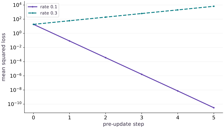
Predict before looking: Which learning rate crosses the stability limit?

Read the figure

The horizontal axis is the pre-update step: step $0$ shows the initial loss before training. The vertical axis is mean squared loss on a logarithmic scale. Both runs start at approximately $18.67$ , but the solid rate- $0.1$ curve falls while the dashed rate- $0.3$ curve rises.

After the first update, the smaller rate gives loss about $0.083$ , whereas the larger rate gives about $60.48$ . By the last plotted step, the losses differ by many orders of magnitude. Equal vertical distances represent equal ratios, not equal absolute changes.

Connect it to the computation

The loss here has curvature $28/3$ . A step multiplies the weight error by $1-\eta(28/3)$ . At rate $0.1$ , this factor is $1/15$ ; at rate $0.3$ , it is $-1.8$ . The larger rate crosses the optimum and increases the error’s magnitude, so squared loss grows by a factor of $3.24$ per update.

The derivative can be correct while the update is unstable. That is the diagnosis this comparison isolates: change the step size before assuming a rising loss proves broken autodiff. The loss curve itself hides the sign alternation; the update equation explains it.

Open full-size figure Download data and provenance

The notebook contains the data experiment, plotting code, and recorded figure output. Rerun it to test your changes.

Where to put & run this code: Work in phases/05-networks/05-debug-unstable-learning/code/main.py (or downloaded exercises/networks-05.py / exercises/networks-05.ipynb) and execute from the repository root with python3 phases/05-networks/05-debug-unstable-learning/code/main.py.

1 Define the controlled objective

Create main.py. Calculate $\operatorname{mean}(x^2)$ and the gradient at $w=0$ before running this block.

main.py · append build step 1

# Step 1 — 1. Define the controlled objective: The initial loss is 56/3 and the initial gradient is -56/3.
import jax
import jax.numpy as jnp
import numpy as np
x=jnp.array([1.,2.,3.])
y=2*x
def loss(w,features=x,targets=y):return jnp.mean((w*features-targets)**2)
def analytic_gradient(w):return (28/3)*(w-2)
np.testing.assert_allclose(loss(0.),56/3,rtol=1e-6)
# Differentiate the objective to obtain gradients ``.
np.testing.assert_allclose(jax.grad(loss)(0.),-56/3,rtol=1e-6)

Code building blocks in this step

jnp.array(values, dtype=...) — Constructs an immutable device-backed JAX array from Python/NumPy values.
x.sum(axis=...) / x.mean(axis=..., keepdims=...) — Reduces values along the named axis (the axis you name is collapsed unless keepdims=True).
jnp.allclose(actual, expected, rtol=..., atol=...) — Checks that two arrays match elementwise within floating-point tolerance.
jax.grad(loss_fn)(params, ...) — Transforms a scalar-output function into a function returning the gradient PyTree with the same structure as params.

The initial loss is $56/3$ and the initial gradient is $-56/3$ . These values independently anchor the autodiff trace.

2 Instrument the update loop

Append the runner. Each history row stores pre-update weight, loss, and gradient magnitude; no optimizer library hides the update.

main.py · append build step 2

# Step 2 — 2. Instrument the update loop: The rate changes while initial state, data, and objective stay fixed.
# Define `run(rate, steps, features, targets...)` to evaluate the objective and its automatic derivatives:
def run(rate,steps,features=x,targets=y,clip=None):
    w=jnp.array(0.)
    history=[]
    objective=lambda value:loss(value,features,targets)
    for _ in range(steps):
        # Differentiate the objective to obtain `(value, grad)` via automatic differentiation.
        value,grad=jax.value_and_grad(objective)(w)
        history.append([float(w),float(value),float(jnp.abs(grad))])
        # Confirm that all computed values remain finite (no NaN or Inf).
        assert np.all(np.isfinite(history[-1]))
        # Combine or mask array elements to form `update`.
        update=jnp.clip(grad,-clip,clip) if clip is not None else grad
        w=w-rate*update
    return float(w),np.asarray(history)
stable,good=run(.1,6)
unstable,bad=run(.3,6)
assert abs(stable-2)<1e-5 and bad[-1,1]>bad[0,1]*100

Code building blocks in this step

jnp.array(values, dtype=...) — Constructs an immutable device-backed JAX array from Python/NumPy values.
jnp.isfinite(x) — Returns a boolean mask verifying that no element is NaN or Inf.
jax.value_and_grad(loss_fn)(params, ...) — Evaluates both the scalar loss and its gradient PyTree (loss_val, grads) in a single forward+backward pass.

The rate changes while initial state, data, and objective stay fixed. This isolates the intervention.

3 Match the recorded failure to the exact recurrence

Append analytic comparisons for every recorded iteration, then print the finite divergence trace.

main.py · append build step 3

# Step 3 — 3. Match the recorded failure to the exact recurrence: An alternating parameter error and a 3.24 loss multiplier support...
for rate,history in [(.1,good),(.3,bad)]:
    expected_w=2-2*(1-rate*28/3)**np.arange(len(history))
    expected_loss=(14/3)*(expected_w-2)**2
    np.testing.assert_allclose(history[:,0],expected_w,rtol=2e-5,atol=1e-5)
    np.testing.assert_allclose(history[:,1],expected_loss,rtol=2e-5,atol=1e-8)
np.testing.assert_allclose(bad[1:,1]/bad[:-1,1],3.24,rtol=1e-5)
print('Stable final weight:',stable,'unstable pre-update [weight,loss,|gradient|]:\n',bad)

Code building blocks in this step

jnp.allclose(actual, expected, rtol=..., atol=...) — Checks that two arrays match elementwise within floating-point tolerance.

An alternating parameter error and a $3.24$ loss multiplier support the learning-rate diagnosis. Near zero, float32 cancellation makes relative loss error misleading, so the analytic comparison uses a $10^{-8}$ absolute floor. No timing or accelerator result is claimed.

View the cumulative build in main.py

These blocks append in order to the same file.

main.py · cumulative Python build

# Step 1 — 1. Define the controlled objective: The initial loss is 56/3 and the initial gradient is -56/3.
import jax
import jax.numpy as jnp
import numpy as np
x=jnp.array([1.,2.,3.])
y=2*x
def loss(w,features=x,targets=y):return jnp.mean((w*features-targets)**2)
def analytic_gradient(w):return (28/3)*(w-2)
np.testing.assert_allclose(loss(0.),56/3,rtol=1e-6)
# Differentiate the objective to obtain gradients ``.
np.testing.assert_allclose(jax.grad(loss)(0.),-56/3,rtol=1e-6)

# Step 2 — 2. Instrument the update loop: The rate changes while initial state, data, and objective stay fixed.
# Define `run(rate, steps, features, targets...)` to evaluate the objective and its automatic derivatives:
def run(rate,steps,features=x,targets=y,clip=None):
    w=jnp.array(0.)
    history=[]
    objective=lambda value:loss(value,features,targets)
    for _ in range(steps):
        # Differentiate the objective to obtain `(value, grad)` via automatic differentiation.
        value,grad=jax.value_and_grad(objective)(w)
        history.append([float(w),float(value),float(jnp.abs(grad))])
        # Confirm that all computed values remain finite (no NaN or Inf).
        assert np.all(np.isfinite(history[-1]))
        # Combine or mask array elements to form `update`.
        update=jnp.clip(grad,-clip,clip) if clip is not None else grad
        w=w-rate*update
    return float(w),np.asarray(history)
stable,good=run(.1,6)
unstable,bad=run(.3,6)
assert abs(stable-2)<1e-5 and bad[-1,1]>bad[0,1]*100

# Step 3 — 3. Match the recorded failure to the exact recurrence: An alternating parameter error and a 3.24 loss multiplier support...
for rate,history in [(.1,good),(.3,bad)]:
    expected_w=2-2*(1-rate*28/3)**np.arange(len(history))
    expected_loss=(14/3)*(expected_w-2)**2
    np.testing.assert_allclose(history[:,0],expected_w,rtol=2e-5,atol=1e-5)
    np.testing.assert_allclose(history[:,1],expected_loss,rtol=2e-5,atol=1e-8)
np.testing.assert_allclose(bad[1:,1]/bad[:-1,1],3.24,rtol=1e-5)
print('Stable final weight:',stable,'unstable pre-update [weight,loss,|gradient|]:\n',bad)

Run the example

python3 phases/05-networks/05-debug-unstable-learning/code/main.py

About this command

This shortcut uses an activated macOS/Linux course environment in the repository folder. For Windows, use the explicit interpreter command in “Setup help” above. The script includes worked examples and reference solutions.

Inspect the complete assembled example

main.py · complete Python example

# Step 1 — 1. Define the controlled objective: The initial loss is 56/3 and the initial gradient is -56/3.
import jax
import jax.numpy as jnp
import numpy as np
x=jnp.array([1.,2.,3.])
y=2*x
def loss(w,features=x,targets=y):return jnp.mean((w*features-targets)**2)
def analytic_gradient(w):return (28/3)*(w-2)
np.testing.assert_allclose(loss(0.),56/3,rtol=1e-6)
# Differentiate the objective to obtain gradients ``.
np.testing.assert_allclose(jax.grad(loss)(0.),-56/3,rtol=1e-6)

# Step 2 — 2. Instrument the update loop: The rate changes while initial state, data, and objective stay fixed.
# Define `run(rate, steps, features, targets...)` to evaluate the objective and its automatic derivatives:
def run(rate,steps,features=x,targets=y,clip=None):
    w=jnp.array(0.)
    history=[]
    objective=lambda value:loss(value,features,targets)
    for _ in range(steps):
        # Differentiate the objective to obtain `(value, grad)` via automatic differentiation.
        value,grad=jax.value_and_grad(objective)(w)
        history.append([float(w),float(value),float(jnp.abs(grad))])
        # Confirm that all computed values remain finite (no NaN or Inf).
        assert np.all(np.isfinite(history[-1]))
        # Combine or mask array elements to form `update`.
        update=jnp.clip(grad,-clip,clip) if clip is not None else grad
        w=w-rate*update
    return float(w),np.asarray(history)
stable,good=run(.1,6)
unstable,bad=run(.3,6)
assert abs(stable-2)<1e-5 and bad[-1,1]>bad[0,1]*100

# Step 3 — 3. Match the recorded failure to the exact recurrence: An alternating parameter error and a 3.24 loss multiplier support...
for rate,history in [(.1,good),(.3,bad)]:
    expected_w=2-2*(1-rate*28/3)**np.arange(len(history))
    expected_loss=(14/3)*(expected_w-2)**2
    np.testing.assert_allclose(history[:,0],expected_w,rtol=2e-5,atol=1e-5)
    np.testing.assert_allclose(history[:,1],expected_loss,rtol=2e-5,atol=1e-8)
np.testing.assert_allclose(bad[1:,1]/bad[:-1,1],3.24,rtol=1e-5)
print('Stable final weight:',stable,'unstable pre-update [weight,loss,|gradient|]:\n',bad)

Expected result: Rate $0.1$ approaches weight $2$ . Rate $0.3$ produces alternating growing errors; consecutive unstable losses have ratio $3.24$ before overflow.

Recorded reference execution

Reference output captured from executing the complete lesson script (code/main.py) and its assertions in the course CPU environment.

2026-10-20T10:46:28.762700+00:00 · Python 3.14.3 · JAX 0.9.2 · 1 CPU device

Stable final weight: 1.999999761581421 unstable pre-update [weight,loss,|gradient|]:
 [[ 0.00000000e+00  1.86666679e+01  1.86666679e+01]
 [ 5.60000038e+00  6.04800110e+01  3.36000061e+01]
 [-4.48000145e+00  1.95955292e+02  6.04800148e+01]
 [ 1.36640034e+01  6.34895264e+02  1.08864037e+02]
 [-1.89952106e+01  2.05706152e+03  1.95955322e+02]
 [ 3.97913895e+01  6.66488281e+03  3.52719635e+02]]
Stable final weight: 1.999999761581421 unstable pre-update [weight,loss,|gradient|]:
 [[ 0.00000000e+00  1.86666679e+01  1.86666679e+01]
 [ 5.60000038e+00  6.04800110e+01  3.36000061e+01]
 [-4.48000145e+00  1.95955292e+02  6.04800148e+01]
 [ 1.36640034e+01  6.34895264e+02  1.08864037e+02]
 [-1.89952106e+01  2.05706152e+03  1.95955322e+02]
 [ 3.97913895e+01  6.66488281e+03  3.52719635e+02]]
Reference / compensated / unchanged-rate updates: 1.8833334 1.8833332 8.416667
PASS: networks-05

Download execution record · The notebook includes executed cells and figure outputs. Compare your run with these values; timings depend on the machine.

Bounded clipped updates

Bounded clipped updates · Python experiment

# Experiment — Bounded clipped updates: Clipping changes the effective update.
clipped,clipped_history=run(.3,6,clip=1.)
assert np.all(np.abs(np.diff(clipped_history[:,0]))<=.300001)
assert clipped_history[-1,1]<clipped_history[0,1]
assert clipped_history[0,2]>1.

Expected: Each recorded displacement is at most $0.3$ while the original gradient norm initially exceeds one.

Clipping changes the effective update. Its boundedness is a useful invariant, not proof of optimal training.

Feature scaling changes curvature

Feature scaling changes curvature · Python experiment

# Experiment — Feature scaling changes curvature: The gradient multiplies by 100 because both prediction and...
scaled_final,scaled=run(.1,3,x*10,y*10)
assert scaled[-1,1]>scaled[0,1]
adjusted_final,adjusted=run(.001,6,x*10,y*10)
np.testing.assert_allclose(adjusted[:,0],good[:,0],rtol=1e-5,atol=1e-5)
np.testing.assert_allclose(adjusted[:,1],good[:,1]*100,rtol=1e-4,atol=1e-8)

Expected: Rate $0.1$ diverges after scaling. Dividing the rate by $100$ restores the original weight trajectory.

The gradient multiplies by $100$ because both prediction and target are scaled; adjusting rate compensates for this fixture.

Hands-On Exercise · Modify & Verify Run in the declared lesson environment

Make it yours

Where to put your code: Append your solution at the bottom of phases/05-networks/05-debug-unstable-learning/code/main.py (or inside the Make it yours cell of exercises/networks-05.ipynb) and run python3 phases/05-networks/05-debug-unstable-learning/code/main.py to verify your prediction before opening the reference solution.

Use features $[1, 1, 1]$ and targets $2$ . Predict the new stability ceiling. Compare stable rate $0.5$ and unstable rate $1.1$ .

Show a writing guide and starter scaffold

How to write this exercise code: step-by-step recipe & starter scaffold

1. Key functions & syntax to use:

jnp.zeros / jnp.ones(shape, dtype=...) — Allocates a tensor of the given shape initialized with constants.
jnp.allclose(actual, expected, rtol=..., atol=...) — Checks that two arrays match elementwise within floating-point tolerance.

2. Step-by-step implementation plan:

Set up the changed input or configuration parameters requested in the prompt.
Run the target function or transformation and assert that the output matches your prediction.

Starter code scaffold · copy into your file & fill in the TODOs

# Exercise solution: Use features [1, 1, 1] and targets 2.
ones = jnp.ones(...)  # TODO: compute ones
exact,history = run(...)  # TODO: compute exact,history
divergent,divergent_history = run(...)  # TODO: compute divergent,divergent_history
np.testing.assert_allclose(exact,2.,atol = ...  # TODO: compute np.testing.assert_allclose(exact,2.,atol
assert divergent_history[-1,1]  # TODO: complete assertion check
np.testing.assert_allclose(divergent_history[1:,1]/divergent_history[:-1,1],1.44,rtol=1e-5)

Reveal the reference solution

Reference solution

# Exercise solution: Use features [1, 1, 1] and targets 2.
ones=jnp.ones(3)
exact,history=run(.5,3,ones,2*ones)
divergent,divergent_history=run(1.1,6,ones,2*ones)
np.testing.assert_allclose(exact,2.,atol=1e-6)
assert divergent_history[-1,1]>divergent_history[0,1]
np.testing.assert_allclose(divergent_history[1:,1]/divergent_history[:-1,1],1.44,rtol=1e-5)

Rescale the objective and compensate the update

Transfer

Multiply the squared-loss objective by five. Compare one plain gradient-descent update at the old rate and at one fifth of that rate. Explain why this compensation does not automatically describe Adam or clipping.

Show a writing guide and starter scaffold

How to write this practice solution: step-by-step recipe & starter scaffold

1. Key functions & syntax to use:

jnp.array(values, dtype=...) — Constructs an immutable device-backed JAX array from Python/NumPy values.
jnp.allclose(actual, expected, rtol=..., atol=...) — Checks that two arrays match elementwise within floating-point tolerance.
jax.grad(loss_fn)(params, ...) — Transforms a scalar-output function into a function returning the gradient PyTree with the same structure as params.

2. Step-by-step implementation plan:

Differentiate the objective to obtain base_gradient via automatic differentiation.
Differentiate the objective to obtain scaled_gradient via automatic differentiation.

Starter code scaffold · copy into your file & fill in the TODOs

# Rescale the objective and compensate the update (Transfer): Scaling the objective scales the gradient.
w0 = jnp.array(...)  # TODO: compute w0
# Differentiate the objective to obtain `base_gradient` via automatic differentiation.
base_gradient = jax.grad(...)  # TODO: compute base_gradient
# Differentiate the objective to obtain `scaled_gradient` via automatic differentiation.
scaled_gradient = jax.grad(...)  # TODO: compute scaled_gradient
np.testing.assert_allclose(scaled_gradient,5*base_gradient,rtol=1e-6)
reference = ...  # TODO: compute reference
compensated = ...  # TODO: compute compensated
uncompensated = ...  # TODO: compute uncompensated
np.testing.assert_allclose(compensated,reference,rtol = ...  # TODO: compute np.testing.assert_allclose(compensated,reference,rtol
assert not np.isclose(uncompensated,reference)  # TODO: complete assertion check
print('Reference / compensated / unchanged-rate updates:',reference,compensated,uncompensated)

Show a hint

Differentiate the scaled objective; plain gradient descent multiplies its gradient by the learning rate.

Reveal reference solution and reasoning

Rescale the objective and compensate the update · Python solution

# Rescale the objective and compensate the update (Transfer): Scaling the objective scales the gradient.
w0=jnp.array(.25)
# Differentiate the objective to obtain `base_gradient` via automatic differentiation.
base_gradient=jax.grad(loss)(w0)
# Differentiate the objective to obtain `scaled_gradient` via automatic differentiation.
scaled_gradient=jax.grad(lambda w:5*loss(w))(w0)
np.testing.assert_allclose(scaled_gradient,5*base_gradient,rtol=1e-6)
reference=w0-.1*base_gradient
compensated=w0-(.1/5)*scaled_gradient
uncompensated=w0-.1*scaled_gradient
np.testing.assert_allclose(compensated,reference,rtol=1e-6)
assert not np.isclose(uncompensated,reference)
print('Reference / compensated / unchanged-rate updates:',reference,compensated,uncompensated)

Scaling the objective scales the gradient. For this plain update the inverse rate change cancels it exactly. Stateful normalization, clipping and regularization need their own analysis.

Diagnose a nonfinite input before an update

Intermediate

Insert one NaN feature. Show that loss/gradient finite checks fail, then repair the source data and recheck the independent initial gradient.

Show a writing guide and starter scaffold

How to write this practice solution: step-by-step recipe & starter scaffold

1. Key functions & syntax to use:

jnp.array(values, dtype=...) — Constructs an immutable device-backed JAX array from Python/NumPy values.
jnp.allclose(actual, expected, rtol=..., atol=...) — Checks that two arrays match elementwise within floating-point tolerance.
jnp.isfinite(x) — Returns a boolean mask verifying that no element is NaN or Inf.
jax.value_and_grad(loss_fn)(params, ...) — Evaluates both the scalar loss and its gradient PyTree (loss_val, grads) in a single forward+backward pass.

2. Step-by-step implementation plan:

Diagnose a nonfinite input before an update (Intermediate): Nonfinite data is a different cause than excessive step size.
Differentiate the objective to obtain (bad_value, bad_grad) via automatic differentiation.
Confirm that all computed values remain finite (no NaN or Inf).
Differentiate the objective to obtain (repaired_value, repaired_grad) via automatic differentiation.
Confirm that all computed values remain finite (no NaN or Inf).

Starter code scaffold · copy into your file & fill in the TODOs

# Diagnose a nonfinite input before an update (Intermediate): Nonfinite data is a different cause than excessive step size.
corrupted = ...  # TODO: compute corrupted
# Differentiate the objective to obtain `(bad_value, bad_grad)` via automatic differentiation.
bad_value,bad_grad = jax.value_and_grad(...)  # TODO: compute bad_value,bad_grad
# Confirm that all computed values remain finite (no NaN or Inf).
assert not np.isfinite(float(bad_value))  # TODO: complete assertion check
repaired = jnp.array(...)  # TODO: compute repaired
# Differentiate the objective to obtain `(repaired_value, repaired_grad)` via automatic differentiation.
repaired_value,repaired_grad = jax.value_and_grad(...)  # TODO: compute repaired_value,repaired_grad
np.testing.assert_allclose(repaired_grad,-56/3,rtol=1e-6)
# Confirm that all computed values remain finite (no NaN or Inf).
assert np.isfinite(float(repaired_value))  # TODO: complete assertion check

Show a hint

Changing the learning rate cannot make a NaN observation valid.

Reveal reference solution and reasoning

Diagnose a nonfinite input before an update · Python solution

# Diagnose a nonfinite input before an update (Intermediate): Nonfinite data is a different cause than excessive step size.
corrupted=x.at[1].set(jnp.nan)
# Differentiate the objective to obtain `(bad_value, bad_grad)` via automatic differentiation.
bad_value,bad_grad=jax.value_and_grad(lambda w:loss(w,corrupted,y))(0.)
# Confirm that all computed values remain finite (no NaN or Inf).
assert not np.isfinite(float(bad_value)) and not np.isfinite(float(bad_grad))
repaired=jnp.array([1.,2.,3.])
# Differentiate the objective to obtain `(repaired_value, repaired_grad)` via automatic differentiation.
repaired_value,repaired_grad=jax.value_and_grad(lambda w:loss(w,repaired,y))(0.)
np.testing.assert_allclose(repaired_grad,-56/3,rtol=1e-6)
# Confirm that all computed values remain finite (no NaN or Inf).
assert np.isfinite(float(repaired_value))

Nonfinite data is a different cause than excessive step size. Repair it at ingestion and validate the objective before taking another update.

Diagnose the result

Start with finite input and loss checks, then inspect shape contracts and independent objective values. Record gradient norm, parameter norm, learning rate, and step index. Alternating growing errors can support a curvature diagnosis; NaNs from corrupted inputs require data repair. Preserve separate train and held-out metrics before declaring the fix successful.

Carry forward

Derive the gradient and curvature on paper
Record pre-update and post-update quantities distinctly
Use gradient clipping for a bounded symptom, not a diagnosis
Change the feature scale and predict the new bound

Keep your evidence

Download evidence template

Keep the analytic error recurrence, per-step weight/loss/gradient norm for rates 0.1 and 0.3, observed 3.24 loss multiplier, changed-scale comparison, clipping bound, and one repaired nonfinite-input case.

Save your modified code, its output, and an explanation of your prediction. Checkpoint answers and exercise evidence are tracked separately.

Saved in this browser. Export or back up your portfolio anytime in My learning.

Save work for this lesson

Verified on local CPU. Stage to a Cloud TPU VM via Cloud TPU setup to record accelerator execution receipts (TODO: add automated Cloud TPU CI execution receipts).

Primary references

Phase 05 Integration Project

Bring this phase together: Build and audit a neural classifier

Checkpoint to prove: Keep train and evaluation behavior separate and reproduce metrics from a saved configuration.

Copy projects/mlp-classifier/starter/model.py to projects/mlp-classifier/my_model.py and write your code in projects/mlp-classifier/my_model.py. Run python3 projects/mlp-classifier/tests/check.py --implementation projects/mlp-classifier/my_model.py --stage 1 from the top-level folder to verify all 3 stages.

Open project workspace Read project guide & figures

Debug unstable learning

What you will be able to do

The problem

The idea

Locate the first broken boundary

Derive the gradient and curvature on paper

Record pre-update and post-update quantities distinctly

Use gradient clipping for a bounded symptom, not a diagnosis

Change the feature scale and predict the new bound

Correct gradients can still produce unstable training

Read the figure

Connect it to the computation

1 Define the controlled objective

2 Instrument the update loop

3 Match the recorded failure to the exact recurrence

Run the example

Recorded reference execution

Bounded clipped updates

Feature scaling changes curvature

Make it yours

Rescale the objective and compensate the update

Diagnose a nonfinite input before an update

Check your understanding

Diagnose the result

Carry forward

Keep your evidence

Primary references

Bring this phase together: Build and audit a neural classifier