Domain Specialization · Local CPULaptop CPULesson 1 of 4 in Phase 11

Phase 11 / Probabilistic modeling

Distributions and sampling

Revision v0.7.0 · 2026-10-20

Lesson · about 90 minutes · CPU practice

Distinguish samples, density, variance and standard error Check normal moments against independent analytic expectations

Phase study guide: preparation, milestones and project evidence

Before you start

Before this: Math & optimization
Hardware: CPU

Download notebook

Other downloads

Python worked examples Lesson text

Setup help: Python, notebook, or Cloud TPU VM

Use the tested CPU packages (the recorded environment uses Python 3.14.3). Other Python versions and accelerator environments require separate checks. The optional Cloud TPU specialization explains the target-specific execution boundaries. Logical CPU devices practice partitioning; they do not simulate TPU performance.

Download the repository ZIP or use your existing checkout. Extract it and open a terminal in the folder containing requirements-cpu.txt. The beginner ZIP is separate; these lessons use the full repository folder.

macOS / Linux terminal · repository folder

python3 -m venv .venv
source .venv/bin/activate
python -m pip install -r requirements-cpu.txt

PowerShell · repository folder

py -3 -m venv .venv
.\.venv\Scripts\python.exe -m pip install -r requirements-cpu.txt

After activation, run the complete worked example from that same folder:

macOS / Linux terminal · activated environment

python phases/11-probability/01-distributions-and-sampling/code/main.py

PowerShell command · repository folder

.\.venv\Scripts\python.exe phases/11-probability/01-distributions-and-sampling/code/main.py

For an incremental build, create main.py in your own practice folder, append each build block in order, and run python main.py with this environment active. Keep that file separate from the downloaded reference solution.

Download this lesson’s notebook. Open it with a Python kernel using the course environment. Run cells from the top after restarting the kernel; experiments depend on earlier definitions.

For local Jupyter, first install the course requirements using the Local Python steps, then use your environment’s Python to start Jupyter:

macOS / Linux terminal · activated course environment

python -m pip install jupyterlab
python -m jupyter lab

PowerShell command · repository folder

.\.venv\Scripts\python.exe -m pip install jupyterlab
.\.venv\Scripts\python.exe -m jupyter lab

Select the downloaded probability-01.ipynb file in JupyterLab. The notebook contains reference solutions; make your prediction and attempt each practice task before opening them. Restart the kernel before changing logical device setup.

Check: The sample mean is close to $2$ , the variance is close to $9$ , and the stable mixture log-density is approximately $-1000.38$ .

Revisit the guided CPU setup · Open 19: TPU Setup. Package instructions are CPU instructions; Windows and accelerator environments need their own validation.

Phase 11.01 Stage 1 of 5 · Understand

1 Understand 2 Build & Run 3 Experiment 4 Exercise & Check 5 Evidence

What you will be able to do

Distinguish samples, density, variance and standard error
Check normal moments against independent analytic expectations
Use log-space arithmetic for an extreme mixture likelihood
Demonstrate both key replay and independent split-key draws

The problem

A sensor model says that a future reading has mean $2$ and standard deviation $3$ . What should a finite collection of simulated readings look like, and how can we check our simulator? We will compare independent formulas with JAX samples, then deliberately underflow a likelihood calculation. This is the numerical foundation for the Bayesian model in the next lesson.

The idea

A distribution describes variability in outcomes. Averaging independent observations can reduce uncertainty in their mean without removing the spread of individual outcomes. Keep these two uncertainties on separate labels and scales.

A precise mean does not make individual outcomes predictable

Suppose observations have standard deviation $2$ . For $100$ independent observations from the same distribution, the sample mean's standard deviation is $2/\sqrt{100}=0.2$ . A new individual observation still has standard deviation $2$ .

The standard-error curve is calculated under its sampling assumptions; it is not itself a collection of measured repeated experiments. Correlated observations can reduce the amount of independent information in a batch.

When interpreting a narrow interval, ask what random quantity the interval describes: a mean, a latent parameter or a new observation. More data can make an estimated average precise while the underlying process remains noisy.

Start with units, not an API

A standard deviation has the same units as a sensor reading. Variance has squared units. To change a standard-normal draw $z$ into a reading, multiply by the standard deviation and add the mean: $x=2+3z$ . The expected variance is $9$ , not $3$ . This is why the scale parameter in our log-density divides the residual before squaring. We assume a strictly positive finite scale; validation belongs at a public input boundary.

p(x\mid\mu,\sigma)=\frac{1}{\sigma\sqrt{2\pi}}\exp\!\left[-\frac12\left(\frac{x-\mu}{\sigma}\right)^2\right],\quad \sigma>0

One draw and a sample average answer different questions

A single future reading has standard deviation $3$ . An average of $N$ independent readings has standard error $3/\sqrt{N}$ . More simulation improves an estimate of the model mean; it does not make the next sensor reading less noisy. At $N=20000$ , the mean standard error is about $0.0212$ . Our deterministic seeded test uses a generous five-standard-error bound and a separate variance check. A statistical tolerance can fail by chance for other seeds, so keep the seed, sample size and actual discrepancy.

Logarithms preserve ratios that densities lose

A normal log-density is a negative quadratic plus normalization terms. Summing log-densities for independent observations avoids multiplying many small values. A mixture is different: it adds weighted densities, so we use log-sum-exp rather than summing component log-densities. For equal components with log-densities $-1000$ and $-1001$ , subtracting the maximum before exponentiation preserves their relative contribution. The ordinary density may still be too small to represent, but its log remains finite.

\log\!\left(\frac{e^a+e^b}{2}\right)=m+\log(e^{a-m}+e^{b-m})-\log 2,\quad m=\max(a,b)

A random key is part of the experiment

Calling a random function twice with the same key and shape replays the same values in this tested environment. It does not create two independent samples. Split the key before assigning it to separate draws. NumPy and JAX need not return matching random arrays for the same integer seed: compare distributional properties, not bit patterns across libraries. Our sample checks establish a small numerical example, not a universal test of a random-number generator.

A precise mean does not remove observation noise

Predict before looking: Which band shrinks when we increase the number of independent observations?

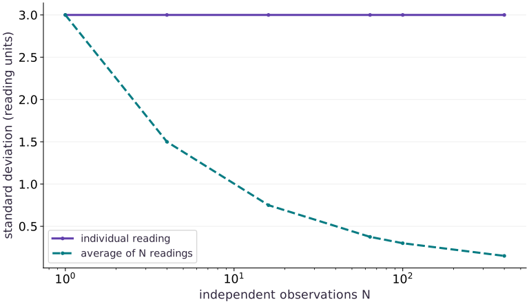
Read the figure

The horizontal axis is the number of independent observations on a logarithmic scale: equal spacing represents equal ratios of sample sizes. The vertical axis is the standard deviation in sensor-reading units. The flat curve stays at $3$ : it describes one reading. The decreasing curve is $3/\sqrt{N}$ : it describes the average of $N$ readings. At $N=100$ , the average has standard deviation $0.3$ , ten times smaller than an individual reading. These curves are analytic quantities evaluated by the executed example, not measured coverage intervals.

Connect it to the computation

The two curves explain the mean test in our code. A large simulation can estimate the distribution mean accurately while predictions for new sensor values remain noisy. Correlated draws, such as the Markov chains later in this phase, do not satisfy the same independent-sample calculation unchanged.

Open full-size figure Download data and provenance

The notebook contains the data experiment, plotting code, and recorded figure output. Rerun it to test your changes.

Where to put & run this code: Work in phases/11-probability/01-distributions-and-sampling/code/main.py (or downloaded exercises/probability-01.py / exercises/probability-01.ipynb) and execute from the repository root with python3 phases/11-probability/01-distributions-and-sampling/code/main.py.

1 Define a density and its contract

Create main.py in the activated CPU environment. Add the imports and the scalar normal log-density. A scale is a positive standard deviation, not a variance.

main.py · append build step 1

# Step 1 — 1. Define a density and its contract: The normalization term matters when comparing different scales;...
import math
import numpy as np
import jax
import jax.numpy as jnp
from jax.scipy.special import logsumexp

def normal_logpdf(value, loc, scale):
    return -0.5*((value-loc)/scale)**2 - jnp.log(scale) - 0.5*jnp.log(2*jnp.pi)

Code building blocks in this step

normal_logpdf(...) — Call normal_logpdf with your updated parameters or inputs from this lesson's workspace.
jnp.log(...) — Call jnp.log with your updated parameters or inputs from this lesson's workspace.

The normalization term matters when comparing different scales; the squared residual alone is not a density.

2 Sample with explicit ownership

Append the sampler. Split one parent key before drawing two samples; retain each array so replay and variation can be checked.

main.py · append build step 2

# Step 2 — 2. Sample with explicit ownership: The broad mean bound is five analytic standard errors for this...
# Create or split explicit PRNG key(s) (`(key_a, key_b)`) for reproducible randomness.
key_a, key_b = jax.random.split(jax.random.key(23))
# Sample deterministic random values into `a` using an explicit PRNG key.
a = 2. + 3.*jax.random.normal(key_a, (20000,))
# Sample deterministic random values into `b` using an explicit PRNG key.
b = 2. + 3.*jax.random.normal(key_b, (20000,))
expected_mean, expected_variance = 2., 9.
assert abs(float(a.mean())-expected_mean) < 5*3/math.sqrt(a.size)
assert abs(float(a.var())-expected_variance) < .4
assert not jnp.array_equal(a,b)
assert jnp.array_equal(a, 2.+3.*jax.random.normal(key_a,(20000,)))

Code building blocks in this step

x.sum(axis=...) / x.mean(axis=..., keepdims=...) — Reduces values along the named axis (the axis you name is collapsed unless keepdims=True).
jax.random.PRNGKey(seed) & jax.random.split(key) — Manages explicit, stateless PRNG keys—always split a key before passing subkeys into independent random draws.

The broad mean bound is five analytic standard errors for this independent normal sample; it is not a guarantee for arbitrary Monte Carlo samples.

3 Compare an independent calculation

Append the independent scalar reference and stable mixture calculation, then run python main.py. Inspect the density, mean and variance.

main.py · append build step 3

# Step 3 — 3. Compare an independent calculation: A log density near negative one thousand remains representable...
actual = normal_logpdf(jnp.array([2.,5.]),2.,3.)
reference = [-math.log(3*math.sqrt(2*math.pi)), -.5-math.log(3*math.sqrt(2*math.pi))]
np.testing.assert_allclose(actual,reference,rtol=1e-6)
components = jnp.array([-1000.,-1001.])
# Evaluate numerically stable log-space cross-entropy/likelihood (`stable`).
stable = logsumexp(components)-jnp.log(2.)
# Confirm that all computed values remain finite (no NaN or Inf).
assert jnp.isfinite(stable)
assert jnp.isneginf(jnp.log(jnp.exp(components).mean()))
print('sample mean, variance:',float(a.mean()),float(a.var()))
print('stable equal-mixture log density:',float(stable))

Code building blocks in this step

jnp.array(values, dtype=...) — Constructs an immutable device-backed JAX array from Python/NumPy values.
x.sum(axis=...) / x.mean(axis=..., keepdims=...) — Reduces values along the named axis (the axis you name is collapsed unless keepdims=True).
jnp.allclose(actual, expected, rtol=..., atol=...) — Checks that two arrays match elementwise within floating-point tolerance.
jnp.isfinite(x) — Returns a boolean mask verifying that no element is NaN or Inf.

A log density near negative one thousand remains representable even when exponentiating it underflows in float32.

View the cumulative build in main.py

These blocks append in order to the same file.

main.py · cumulative Python build

# Step 1 — 1. Define a density and its contract: The normalization term matters when comparing different scales;...
import math
import numpy as np
import jax
import jax.numpy as jnp
from jax.scipy.special import logsumexp

def normal_logpdf(value, loc, scale):
    return -0.5*((value-loc)/scale)**2 - jnp.log(scale) - 0.5*jnp.log(2*jnp.pi)

# Step 2 — 2. Sample with explicit ownership: The broad mean bound is five analytic standard errors for this...
# Create or split explicit PRNG key(s) (`(key_a, key_b)`) for reproducible randomness.
key_a, key_b = jax.random.split(jax.random.key(23))
# Sample deterministic random values into `a` using an explicit PRNG key.
a = 2. + 3.*jax.random.normal(key_a, (20000,))
# Sample deterministic random values into `b` using an explicit PRNG key.
b = 2. + 3.*jax.random.normal(key_b, (20000,))
expected_mean, expected_variance = 2., 9.
assert abs(float(a.mean())-expected_mean) < 5*3/math.sqrt(a.size)
assert abs(float(a.var())-expected_variance) < .4
assert not jnp.array_equal(a,b)
assert jnp.array_equal(a, 2.+3.*jax.random.normal(key_a,(20000,)))

# Step 3 — 3. Compare an independent calculation: A log density near negative one thousand remains representable...
actual = normal_logpdf(jnp.array([2.,5.]),2.,3.)
reference = [-math.log(3*math.sqrt(2*math.pi)), -.5-math.log(3*math.sqrt(2*math.pi))]
np.testing.assert_allclose(actual,reference,rtol=1e-6)
components = jnp.array([-1000.,-1001.])
# Evaluate numerically stable log-space cross-entropy/likelihood (`stable`).
stable = logsumexp(components)-jnp.log(2.)
# Confirm that all computed values remain finite (no NaN or Inf).
assert jnp.isfinite(stable)
assert jnp.isneginf(jnp.log(jnp.exp(components).mean()))
print('sample mean, variance:',float(a.mean()),float(a.var()))
print('stable equal-mixture log density:',float(stable))

Run the example

python3 phases/11-probability/01-distributions-and-sampling/code/main.py

About this command

This shortcut uses an activated macOS/Linux course environment in the repository folder. For Windows, use the explicit interpreter command in “Setup help” above. The script includes worked examples and reference solutions.

Inspect the complete assembled example

main.py · complete Python example

# Step 1 — 1. Define a density and its contract: The normalization term matters when comparing different scales;...
import math
import numpy as np
import jax
import jax.numpy as jnp
from jax.scipy.special import logsumexp

def normal_logpdf(value, loc, scale):
    return -0.5*((value-loc)/scale)**2 - jnp.log(scale) - 0.5*jnp.log(2*jnp.pi)

# Step 2 — 2. Sample with explicit ownership: The broad mean bound is five analytic standard errors for this...
# Create or split explicit PRNG key(s) (`(key_a, key_b)`) for reproducible randomness.
key_a, key_b = jax.random.split(jax.random.key(23))
# Sample deterministic random values into `a` using an explicit PRNG key.
a = 2. + 3.*jax.random.normal(key_a, (20000,))
# Sample deterministic random values into `b` using an explicit PRNG key.
b = 2. + 3.*jax.random.normal(key_b, (20000,))
expected_mean, expected_variance = 2., 9.
assert abs(float(a.mean())-expected_mean) < 5*3/math.sqrt(a.size)
assert abs(float(a.var())-expected_variance) < .4
assert not jnp.array_equal(a,b)
assert jnp.array_equal(a, 2.+3.*jax.random.normal(key_a,(20000,)))

# Step 3 — 3. Compare an independent calculation: A log density near negative one thousand remains representable...
actual = normal_logpdf(jnp.array([2.,5.]),2.,3.)
reference = [-math.log(3*math.sqrt(2*math.pi)), -.5-math.log(3*math.sqrt(2*math.pi))]
np.testing.assert_allclose(actual,reference,rtol=1e-6)
components = jnp.array([-1000.,-1001.])
# Evaluate numerically stable log-space cross-entropy/likelihood (`stable`).
stable = logsumexp(components)-jnp.log(2.)
# Confirm that all computed values remain finite (no NaN or Inf).
assert jnp.isfinite(stable)
assert jnp.isneginf(jnp.log(jnp.exp(components).mean()))
print('sample mean, variance:',float(a.mean()),float(a.var()))
print('stable equal-mixture log density:',float(stable))

Expected result: The sample mean is close to $2$ , the variance is close to $9$ , and the stable mixture log-density is approximately $-1000.38$ .

Recorded reference execution

Reference output captured from executing the complete lesson script (code/main.py) and its assertions in the course CPU environment.

2026-10-20T10:48:36.575595+00:00 · Python 3.14.3 · JAX 0.9.2 · 1 CPU device

sample mean, variance: 2.0067408084869385 9.035282135009766
stable equal-mixture log density: -1000.3799438476562
sample mean, variance: 2.0067408084869385 9.035282135009766
stable equal-mixture log density: -1000.3799438476562
peak density: 3.9894230365753174
-5.0 -2.379885673522949
PASS: probability-01

Download execution record · The notebook includes executed cells and figure outputs. Compare your run with these values; timings depend on the machine.

Density can exceed one

Density can exceed one · Python experiment

# Experiment — Density can exceed one: A narrow continuous density can exceed one; its area, not its...
peak = jnp.exp(normal_logpdf(0.,0.,.1))
assert peak > 1
print("peak density:",float(peak))

Expected: The peak density is approximately $3.99$ .

A narrow continuous density can exceed one; its area, not its height at a point, sums to one.

Separate sum and mixture

Separate sum and mixture · Python experiment

# Experiment — Separate sum and mixture: Independence multiplies probabilities, while alternative mixture...
values = jnp.array([-2.,-3.])
# Aggregate array values to compute `independent_log`.
independent_log = values.sum()
# Evaluate numerically stable log-space cross-entropy/likelihood (`mixture_log`).
mixture_log = logsumexp(values)-jnp.log(2.)
assert jnp.allclose(independent_log,-5.)
assert mixture_log > -3.
print(float(independent_log),float(mixture_log))

Expected: The independent joint log likelihood is $-5$ ; the mixture log density is approximately $-2.38$ .

Independence multiplies probabilities, while alternative mixture components add weighted probabilities.

Hands-On Exercise · Modify & Verify Run in the declared lesson environment

Make it yours

Where to put your code: Append your solution at the bottom of phases/11-probability/01-distributions-and-sampling/code/main.py (or inside the Make it yours cell of exercises/probability-01.ipynb) and run python3 phases/11-probability/01-distributions-and-sampling/code/main.py to verify your prediction before opening the reference solution.

Change the sensor to mean $-1$ , standard deviation $0.5$ , and draw $30000$ readings from a new key. Predict the variance and the standard error of the sample mean, then verify both moments.

Show a writing guide and starter scaffold

How to write this exercise code: step-by-step recipe & starter scaffold

1. Key functions & syntax to use:

x.sum(axis=...) / x.mean(axis=..., keepdims=...) — Reduces values along the named axis (the axis you name is collapsed unless keepdims=True).
jax.random.PRNGKey(seed) & jax.random.split(key) — Manages explicit, stateless PRNG keys—always split a key before passing subkeys into independent random draws.

2. Step-by-step implementation plan:

Create or split explicit PRNG key(s) (changed) for reproducible randomness.

Starter code scaffold · copy into your file & fill in the TODOs

# Exercise solution: Change the sensor to mean -1, standard deviation 0.5, and draw 30000...
# Create or split explicit PRNG key(s) (`changed`) for reproducible randomness.
changed = ...  # TODO: compute changed
assert abs(float(changed.mean())+1.)  # TODO: complete assertion check
assert abs(float(changed.var())-.25)  # TODO: complete assertion check

Reveal the reference solution

Reference solution

# Exercise solution: Change the sensor to mean -1, standard deviation 0.5, and draw 30000...
# Create or split explicit PRNG key(s) (`changed`) for reproducible randomness.
changed = -1.+.5*jax.random.normal(jax.random.key(51),(30000,))
assert abs(float(changed.mean())+1.) < 5*.5/math.sqrt(30000)
assert abs(float(changed.var())-.25) < .015

Detect a missing normalization

Transfer / diagnosis

Compare scales $1$ and $2$ at their common mean. Show why a residual-only objective incorrectly ties them.

Show a writing guide and starter scaffold

How to write this practice solution: step-by-step recipe & starter scaffold

1. Key functions & syntax to use:

jnp.array(values, dtype=...) — Constructs an immutable device-backed JAX array from Python/NumPy values.
jnp.allclose(actual, expected, rtol=..., atol=...) — Checks that two arrays match elementwise within floating-point tolerance.

2. Step-by-step implementation plan:

Set up the changed input or configuration parameters requested in the prompt.
Run the target function or transformation and assert that the output matches your prediction.

Starter code scaffold · copy into your file & fill in the TODOs

# Detect a missing normalization (Transfer / diagnosis): Scale changes density even with identical zero residuals.
scores = normal_logpdf(...)  # TODO: compute scores
assert jnp.allclose(scores[0]-scores[1],jnp.log(2.))  # TODO: complete assertion check

Show a hint

The residual is zero for both; retain $-\log\sigma$ .

Reveal reference solution and reasoning

Detect a missing normalization · Python solution

# Detect a missing normalization (Transfer / diagnosis): Scale changes density even with identical zero residuals.
scores = normal_logpdf(0.,0.,jnp.array([1.,2.]))
assert jnp.allclose(scores[0]-scores[1],jnp.log(2.))

Scale changes density even with identical zero residuals.

Demonstrate key ownership

Transfer / diagnosis

Produce two separately owned standard-normal draws and show replay of the first. Explain why replay alone does not test independence.

Show a writing guide and starter scaffold

How to write this practice solution: step-by-step recipe & starter scaffold

1. Key functions & syntax to use:

jax.random.PRNGKey(seed) & jax.random.split(key) — Manages explicit, stateless PRNG keys—always split a key before passing subkeys into independent random draws.

2. Step-by-step implementation plan:

Create or split explicit PRNG key(s) ((left, right)) for reproducible randomness.
Sample deterministic random values into first using an explicit PRNG key.
Sample deterministic random values into second using an explicit PRNG key.

Starter code scaffold · copy into your file & fill in the TODOs

# Demonstrate key ownership (Transfer / diagnosis): Different split keys avoid accidental replay; one differing...
# Create or split explicit PRNG key(s) (`(left, right)`) for reproducible randomness.
left,right = jax.random.split(...)  # TODO: compute left,right
# Sample deterministic random values into `first` using an explicit PRNG key.
first = jax.random.normal(...)  # TODO: compute first
# Sample deterministic random values into `second` using an explicit PRNG key.
second = jax.random.normal(...)  # TODO: compute second
assert jnp.array_equal(first,jax.random.normal(left,(32,)))  # TODO: complete assertion check
assert not jnp.array_equal(first,second)  # TODO: complete assertion check

Show a hint

Split before use; compare arrays with the same shape.

Reveal reference solution and reasoning

Demonstrate key ownership · Python solution

# Demonstrate key ownership (Transfer / diagnosis): Different split keys avoid accidental replay; one differing...
# Create or split explicit PRNG key(s) (`(left, right)`) for reproducible randomness.
left,right = jax.random.split(jax.random.key(17))
# Sample deterministic random values into `first` using an explicit PRNG key.
first = jax.random.normal(left,(32,))
# Sample deterministic random values into `second` using an explicit PRNG key.
second = jax.random.normal(right,(32,))
assert jnp.array_equal(first,jax.random.normal(left,(32,)))
assert not jnp.array_equal(first,second)

Different split keys avoid accidental replay; one differing pair does not prove every statistical property of a generator.

Diagnose the result

If the simulated variance is near three instead of nine, inspect whether you multiplied by sqrt $3$ when the stated scale was three. If two supposedly independent arrays match exactly, inspect key reuse before changing the distribution. If a mixture likelihood becomes negative infinity, compare the log-sum-exp result before widening dtype.

Carry forward

A density is not a point probability.
Moment checks need sample size, units and a justified tolerance.
Log-space arithmetic and explicit keys make likelihood experiments inspectable.

Keep your evidence

Download evidence template

Seeded arrays, independent density values, moment discrepancies and underflow diagnosis. Keep the environment, observed outputs and your explanation of the figure.

Save your modified code, its output, and an explanation of your prediction. Checkpoint answers and exercise evidence are tracked separately.

Saved in this browser. Export or back up your portfolio anytime in My learning.

Save work for this lesson

Verified on local CPU. Stage to a Cloud TPU VM via Cloud TPU setup to record accelerator execution receipts (TODO: add automated Cloud TPU CI execution receipts).

Distributions and sampling

What you will be able to do

The problem

The idea

A precise mean does not make individual outcomes predictable

Start with units, not an API

One draw and a sample average answer different questions

Logarithms preserve ratios that densities lose

A random key is part of the experiment

A precise mean does not remove observation noise

Read the figure

Connect it to the computation

1 Define a density and its contract

2 Sample with explicit ownership

3 Compare an independent calculation

Run the example

Recorded reference execution

Density can exceed one

Separate sum and mixture

Make it yours

Detect a missing normalization

Demonstrate key ownership

Check your understanding

Diagnose the result

Carry forward

Keep your evidence

Primary references