Domain Specialization · Local CPULaptop CPULesson 3 of 4 in Phase 11

Phase 11 / Probabilistic modeling

Hamiltonian Monte Carlo and sampler diagnostics

Revision v0.7.0 · 2026-10-20

Lesson · about 140 minutes · CPU practice

Implement leapfrog with the correct half-step boundaries Check reversibility and an independent analytic gradient

Phase study guide: preparation, milestones and project evidence

Before you start

Before this: Build a Bayesian regression
Hardware: CPU

Download notebook

Other downloads

Python worked examples Lesson text

Setup help: Python, notebook, or Cloud TPU VM

Use the tested CPU packages (the recorded environment uses Python 3.14.3). Other Python versions and accelerator environments require separate checks. The optional Cloud TPU specialization explains the target-specific execution boundaries. Logical CPU devices practice partitioning; they do not simulate TPU performance.

Download the repository ZIP or use your existing checkout. Extract it and open a terminal in the folder containing requirements-cpu.txt. The beginner ZIP is separate; these lessons use the full repository folder.

macOS / Linux terminal · repository folder

python3 -m venv .venv
source .venv/bin/activate
python -m pip install -r requirements-cpu.txt

PowerShell · repository folder

py -3 -m venv .venv
.\.venv\Scripts\python.exe -m pip install -r requirements-cpu.txt

After activation, run the complete worked example from that same folder:

macOS / Linux terminal · activated environment

python phases/11-probability/03-hamiltonian-monte-carlo-and-sampler-diagnostics/code/main.py

PowerShell command · repository folder

.\.venv\Scripts\python.exe phases/11-probability/03-hamiltonian-monte-carlo-and-sampler-diagnostics/code/main.py

For an incremental build, create main.py in your own practice folder, append each build block in order, and run python main.py with this environment active. Keep that file separate from the downloaded reference solution.

Download this lesson’s notebook. Open it with a Python kernel using the course environment. Run cells from the top after restarting the kernel; experiments depend on earlier definitions.

For local Jupyter, first install the course requirements using the Local Python steps, then use your environment’s Python to start Jupyter:

macOS / Linux terminal · activated course environment

python -m pip install jupyterlab
python -m jupyter lab

PowerShell command · repository folder

.\.venv\Scripts\python.exe -m pip install jupyterlab
.\.venv\Scripts\python.exe -m jupyter lab

Select the downloaded probability-03.ipynb file in JupyterLab. The notebook contains reference solutions; make your prediction and attempt each practice task before opening them. Restart the kernel before changing logical device setup.

Check: The pooled mean and covariance approach the stated target within the fixture tolerances. The two classical split R-hat values, one per parameter coordinate, remain near $1$ ; acceptance is reported separately for each chain.

Revisit the guided CPU setup · Open 19: TPU Setup. Package instructions are CPU instructions; Windows and accelerator environments need their own validation.

Phase 11.03 Stage 1 of 5 · Understand

1 Understand 2 Build & Run 3 Experiment 4 Exercise & Check 5 Evidence

What you will be able to do

Implement leapfrog with the correct half-step boundaries
Check reversibility and an independent analytic gradient
Compare four seeded chains with a known posterior
Interpret energy error, acceptance and classical split R-hat without claiming convergence

The problem

An approximate inference program returns a long list of weights. Before treating those weights as posterior samples, how can we tell whether its mechanics are correct and whether its chains explored the target? We will build a transparent Hamiltonian Monte Carlo sampler for a correlated Gaussian with a known mean and covariance, then deliberately damage its step size.

The idea

Hamiltonian Monte Carlo introduces momentum to propose distant states while accounting for the target density. Numerical integration and acceptance control the proposal, but diagnostics are still needed to judge whether the retained samples explore the posterior adequately.

A moving chain is not automatically a well-mixed chain

Follow position and momentum through a leapfrog trajectory. A proposal can travel far without behaving like an independent posterior draw. Integration error and acceptance behavior provide one diagnostic, while between-chain agreement and autocorrelation provide others.

Start multiple chains from meaningfully different positions where appropriate. Inspect the same retained sampling region across chains, and separate adaptation from retained draws. A trace that looks active may still stay in one region or be strongly correlated.

The lesson's trace plot uses a known posterior mean as a reference. Matching that mean is not sufficient: spread and dependence matter too. Compute diagnostics from the retained samples with their conventions recorded; plotting a thinned subset should not silently redefine the diagnostic sample.

Turn log-density into potential energy

For a normal target with mean $m$ and covariance $\Sigma$ , the potential is $U(q)=(q-m)^\top\Sigma^{-1}(q-m)/2$ , ignoring a constant. Its gradient is $\Sigma^{-1}(q-m)$ , so we have an independent formula for autodiff. Momentum has a standard-normal distribution and kinetic energy $p^\top p/2$ . The combined energy should remain constant along an exact trajectory.

H(q,p)=U(q)+\tfrac12p^\top p,\qquad \nabla U(q)=\Sigma^{-1}(q-m)

Trace the half steps

First take a half momentum step using the current gradient. Take a full position step with that momentum, then update momentum using the new position. Interior momentum steps are full steps; the final one is a half step. This symmetry gives a reversible integrator up to numerical error. Our check negates the final momentum and integrates again; it should return to the starting position and negative starting momentum. A loop with all full momentum steps fails that boundary test.

Correct discretization error in log space

A proposed trajectory changes energy by $\Delta H$ . Accept with probability $\min(1,e^{-\Delta H})$ , implemented as $\log u<-\Delta H$ . A rejected proposal retains the current sample; removing repeated values would change the distribution. Non-finite energy error is rejected. The signed energy error can be negative, so it should not be interpreted as a nonnegative loss. An enormous positive error suggests an integration problem, often a step size too large for target curvature.

Combine multiple sampler diagnostics

We start four chains from dispersed points and discard the first $400$ transitions. This fixed discard is a teaching convention, not automatic warmup adaptation. Classical split R-hat compares between-chain and within-chain variance after splitting each chain. A value near one says those variance estimates agree; chains can still miss a mode together. Modern rank-normalized split R-hat, bulk and tail effective sample size, Monte Carlo standard errors and divergence diagnostics are stronger complementary tools. Our compact implementation is explicitly classical R-hat and does not implement those modern diagnostics.

Use the reference model to expose failure

Here the exact mean, variance and covariance are known. Check all of them: getting both marginal means right can still hide missing correlation. Acceptance alone is insufficient; a tiny step can accept almost everything while exploring slowly. Effective sample size concerns the information in correlated draws, not the number of rows stored. Before using a library such as NumPyro on an unknown posterior, repeat an exact-model validation and inspect its documented diagnostics. This CPU fixture establishes neither multimodal exploration nor accelerator performance.

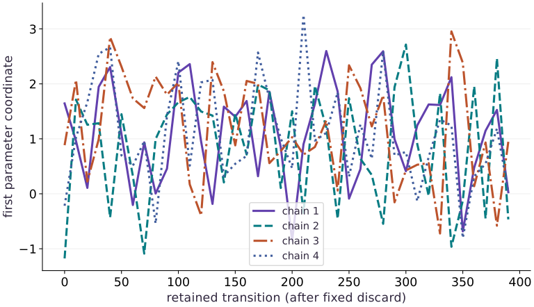
Four HMC traces around a known posterior mean

Predict before looking: Can the chains cross the known mean while still showing successive correlated values?

Read the figure

The horizontal axis counts retained transitions after discarding the initial $400$ . The vertical axis is the first coordinate of the sampled parameter. Each colored line is one chain, plotted at every tenth retained transition to keep the figure readable. The target mean is $1$ ; the chains move on both sides of it. Their paths differ because they use different keys and initial positions. Connecting thinned points helps visual inspection but does not make the underlying draws independent.

Connect it to the computation

This trace is one piece of the evidence. The code also checks the two-dimensional covariance, which a single-coordinate trace cannot show, and prints classical split R-hat and acceptance. A smooth-looking trace or repeated crossings of the mean is distinct from exploration of modes absent from this single-Gaussian fixture.

Open full-size figure Download data and provenance

The notebook contains the data experiment, plotting code, and recorded figure output. Rerun it to test your changes.

Where to put & run this code: Work in phases/11-probability/03-hamiltonian-monte-carlo-and-sampler-diagnostics/code/main.py (or downloaded exercises/probability-03.py / exercises/probability-03.ipynb) and execute from the repository root with python3 phases/11-probability/03-hamiltonian-monte-carlo-and-sampler-diagnostics/code/main.py.

1 Write a known target and its gradient

Create a fresh main.py. This correlated Gaussian is an exact test target for an inference algorithm, not a new unknown statistical model.

main.py · append build step 1

# Step 1 — 1. Write a known target and its gradient: Potential energy is the negative log-density up to a constant,...
import numpy as np
import jax
import jax.numpy as jnp
target_mean = jnp.array([1.,-1.])
target_cov = jnp.array([[1.,.8],[.8,1.]])
precision = jnp.linalg.solve(target_cov,jnp.eye(2))
def potential(q):
    delta=q-target_mean
    return .5*delta@precision@delta
# Differentiate the objective to obtain `force` via automatic differentiation.
force=jax.grad(potential)
assert jnp.allclose(force(jnp.array([0.,0.])),precision@(-target_mean))

Code building blocks in this step

jnp.array(values, dtype=...) — Constructs an immutable device-backed JAX array from Python/NumPy values.
jnp.zeros / jnp.ones(shape, dtype=...) — Allocates a tensor of the given shape initialized with constants.
jnp.allclose(actual, expected, rtol=..., atol=...) — Checks that two arrays match elementwise within floating-point tolerance.
jax.grad(loss_fn)(params, ...) — Transforms a scalar-output function into a function returning the gradient PyTree with the same structure as params.

Potential energy is the negative log-density up to a constant, which cancels in the acceptance ratio.

2 Integrate then accept or reject

Append a leapfrog trajectory and a chain. Every transition splits keys for momentum and acceptance; rejection retains the old position.

main.py · append build step 2

# Step 2 — 2. Integrate then accept or reject: Leapfrog approximates energy conservation.
def leapfrog(q,p,step_size,steps):
    p=p-.5*step_size*force(q)
    def step(i,state):
        q,p=state
        q=q+step_size*p
        # Combine or mask array elements to form `p`.
        p=p-jnp.where(i<steps-1,step_size,.5*step_size)*force(q)
        return q,p
    return jax.lax.fori_loop(0,steps,step,(q,p))

# Define `chain(key, initial, step_size, leapfrog_steps...)` to carry state across steps with `jax.lax.scan`:
def chain(key,initial,step_size=.25,leapfrog_steps=7,draws=1600):
    def transition(state,_):
        q,key=state
        # Create or split explicit PRNG key(s) (`(key, kp, ku)`) for reproducible randomness.
        key,kp,ku=jax.random.split(key,3)
        # Sample deterministic random values into `p` using an explicit PRNG key.
        p=jax.random.normal(kp,q.shape)
        proposal,new_p=leapfrog(q,p,step_size,leapfrog_steps)
        error=potential(proposal)+.5*jnp.sum(new_p**2)-potential(q)-.5*jnp.sum(p**2)
        # Draw pseudorandom samples for `accept` using the explicit RNG state.
        accept=jnp.isfinite(error)&(jnp.log(jax.random.uniform(ku)) < -error)
        # Combine or mask array elements to form `next_q`.
        next_q=jnp.where(accept,proposal,q)
        return (next_q,key),(next_q,accept,error)
    # Run compiled structured control flow via `jax.lax` (`(_, record)`).
    _,record=jax.lax.scan(transition,(initial,key),None,length=draws)
    return record

Code building blocks in this step

x.sum(axis=...) / x.mean(axis=..., keepdims=...) — Reduces values along the named axis (the axis you name is collapsed unless keepdims=True).
jnp.isfinite(x) — Returns a boolean mask verifying that no element is NaN or Inf.
jax.lax.scan(step_fn, init_carry, xs, length=...) — Compiles a sequential loop where step_fn(carry, x) returns (next_carry, y), returning (final_carry, stacked_ys).
jax.random.PRNGKey(seed) & jax.random.split(key) — Manages explicit, stateless PRNG keys—always split a key before passing subkeys into independent random draws.

Leapfrog approximates energy conservation. Metropolis correction removes integration bias in the ideal stationary distribution; it does not make a finite chain independent or guarantee exploration.

3 Compare chains and an analytic oracle

Append four dispersed starts, discard an explicitly fixed initial segment, and retain all diagnostics. Run python main.py.

main.py · append build step 3

# Step 3 — 3. Compare chains and an analytic oracle: The tolerances test this seeded Gaussian fixture only.
starts=jnp.array([[-4.,-4.],[-4.,4.],[4.,-4.],[4.,4.]])
# Create or split explicit PRNG key(s) (`records`) for reproducible randomness.
records=jax.vmap(lambda key,start:chain(key,start))(jax.random.split(jax.random.key(71),4),starts)
samples=records[0][:,400:,:]
def split_rhat(values):
    # Classical split R-hat for one scalar coordinate; not rank-normalized.
    half=values.shape[1]//2
    # Combine or mask array elements to form `split`.
    split=jnp.concatenate([values[:,:half],values[:,-half:]],axis=0)
    # Reduce along axis=1 to compute `within`.
    within=jnp.var(split,axis=1,ddof=1).mean()
    # Reduce along axis=1 to compute `between`.
    between=half*jnp.var(split.mean(axis=1),ddof=1)
    return jnp.sqrt(((half-1)*within/half+between/half)/within)
# Vectorize across the batch dimension with `jax.vmap` (`rhats`).
rhats=jax.vmap(split_rhat,in_axes=2)(samples)
# Construct and reshape `pooled` into the target tensor dimensions.
pooled=samples.reshape(-1,2)
assert jnp.max(jnp.abs(pooled.mean(0)-target_mean))<.15
assert jnp.max(jnp.abs(jnp.cov(pooled.T)-target_cov))<.2
assert jnp.all(rhats<1.05)
print('mean:',pooled.mean(0),'covariance:',jnp.cov(pooled.T))
print('classical split R-hat:',rhats,'acceptance:',records[1].mean(axis=1))

Code building blocks in this step

jnp.array(values, dtype=...) — Constructs an immutable device-backed JAX array from Python/NumPy values.
array.reshape(new_shape) — Reorganizes tensor axes without changing the total element count (array.size).
x.sum(axis=...) / x.mean(axis=..., keepdims=...) — Reduces values along the named axis (the axis you name is collapsed unless keepdims=True).
jax.vmap(fn, in_axes=..., out_axes=...) — Vectorizes a single-example function across a batch axis without writing a Python loop.

The tolerances test this seeded Gaussian fixture only. Agreement with a known posterior is stronger evidence here than a diagnostic threshold alone.

View the cumulative build in main.py

These blocks append in order to the same file.

main.py · cumulative Python build

# Step 1 — 1. Write a known target and its gradient: Potential energy is the negative log-density up to a constant,...
import numpy as np
import jax
import jax.numpy as jnp
target_mean = jnp.array([1.,-1.])
target_cov = jnp.array([[1.,.8],[.8,1.]])
precision = jnp.linalg.solve(target_cov,jnp.eye(2))
def potential(q):
    delta=q-target_mean
    return .5*delta@precision@delta
# Differentiate the objective to obtain `force` via automatic differentiation.
force=jax.grad(potential)
assert jnp.allclose(force(jnp.array([0.,0.])),precision@(-target_mean))

# Step 2 — 2. Integrate then accept or reject: Leapfrog approximates energy conservation.
def leapfrog(q,p,step_size,steps):
    p=p-.5*step_size*force(q)
    def step(i,state):
        q,p=state
        q=q+step_size*p
        # Combine or mask array elements to form `p`.
        p=p-jnp.where(i<steps-1,step_size,.5*step_size)*force(q)
        return q,p
    return jax.lax.fori_loop(0,steps,step,(q,p))

# Define `chain(key, initial, step_size, leapfrog_steps...)` to carry state across steps with `jax.lax.scan`:
def chain(key,initial,step_size=.25,leapfrog_steps=7,draws=1600):
    def transition(state,_):
        q,key=state
        # Create or split explicit PRNG key(s) (`(key, kp, ku)`) for reproducible randomness.
        key,kp,ku=jax.random.split(key,3)
        # Sample deterministic random values into `p` using an explicit PRNG key.
        p=jax.random.normal(kp,q.shape)
        proposal,new_p=leapfrog(q,p,step_size,leapfrog_steps)
        error=potential(proposal)+.5*jnp.sum(new_p**2)-potential(q)-.5*jnp.sum(p**2)
        # Draw pseudorandom samples for `accept` using the explicit RNG state.
        accept=jnp.isfinite(error)&(jnp.log(jax.random.uniform(ku)) < -error)
        # Combine or mask array elements to form `next_q`.
        next_q=jnp.where(accept,proposal,q)
        return (next_q,key),(next_q,accept,error)
    # Run compiled structured control flow via `jax.lax` (`(_, record)`).
    _,record=jax.lax.scan(transition,(initial,key),None,length=draws)
    return record

# Step 3 — 3. Compare chains and an analytic oracle: The tolerances test this seeded Gaussian fixture only.
starts=jnp.array([[-4.,-4.],[-4.,4.],[4.,-4.],[4.,4.]])
# Create or split explicit PRNG key(s) (`records`) for reproducible randomness.
records=jax.vmap(lambda key,start:chain(key,start))(jax.random.split(jax.random.key(71),4),starts)
samples=records[0][:,400:,:]
def split_rhat(values):
    # Classical split R-hat for one scalar coordinate; not rank-normalized.
    half=values.shape[1]//2
    # Combine or mask array elements to form `split`.
    split=jnp.concatenate([values[:,:half],values[:,-half:]],axis=0)
    # Reduce along axis=1 to compute `within`.
    within=jnp.var(split,axis=1,ddof=1).mean()
    # Reduce along axis=1 to compute `between`.
    between=half*jnp.var(split.mean(axis=1),ddof=1)
    return jnp.sqrt(((half-1)*within/half+between/half)/within)
# Vectorize across the batch dimension with `jax.vmap` (`rhats`).
rhats=jax.vmap(split_rhat,in_axes=2)(samples)
# Construct and reshape `pooled` into the target tensor dimensions.
pooled=samples.reshape(-1,2)
assert jnp.max(jnp.abs(pooled.mean(0)-target_mean))<.15
assert jnp.max(jnp.abs(jnp.cov(pooled.T)-target_cov))<.2
assert jnp.all(rhats<1.05)
print('mean:',pooled.mean(0),'covariance:',jnp.cov(pooled.T))
print('classical split R-hat:',rhats,'acceptance:',records[1].mean(axis=1))

Run the example

python3 phases/11-probability/03-hamiltonian-monte-carlo-and-sampler-diagnostics/code/main.py

About this command

This shortcut uses an activated macOS/Linux course environment in the repository folder. For Windows, use the explicit interpreter command in “Setup help” above. The script includes worked examples and reference solutions.

Inspect the complete assembled example

main.py · complete Python example

# Step 1 — 1. Write a known target and its gradient: Potential energy is the negative log-density up to a constant,...
import numpy as np
import jax
import jax.numpy as jnp
target_mean = jnp.array([1.,-1.])
target_cov = jnp.array([[1.,.8],[.8,1.]])
precision = jnp.linalg.solve(target_cov,jnp.eye(2))
def potential(q):
    delta=q-target_mean
    return .5*delta@precision@delta
# Differentiate the objective to obtain `force` via automatic differentiation.
force=jax.grad(potential)
assert jnp.allclose(force(jnp.array([0.,0.])),precision@(-target_mean))

# Step 2 — 2. Integrate then accept or reject: Leapfrog approximates energy conservation.
def leapfrog(q,p,step_size,steps):
    p=p-.5*step_size*force(q)
    def step(i,state):
        q,p=state
        q=q+step_size*p
        # Combine or mask array elements to form `p`.
        p=p-jnp.where(i<steps-1,step_size,.5*step_size)*force(q)
        return q,p
    return jax.lax.fori_loop(0,steps,step,(q,p))

# Define `chain(key, initial, step_size, leapfrog_steps...)` to carry state across steps with `jax.lax.scan`:
def chain(key,initial,step_size=.25,leapfrog_steps=7,draws=1600):
    def transition(state,_):
        q,key=state
        # Create or split explicit PRNG key(s) (`(key, kp, ku)`) for reproducible randomness.
        key,kp,ku=jax.random.split(key,3)
        # Sample deterministic random values into `p` using an explicit PRNG key.
        p=jax.random.normal(kp,q.shape)
        proposal,new_p=leapfrog(q,p,step_size,leapfrog_steps)
        error=potential(proposal)+.5*jnp.sum(new_p**2)-potential(q)-.5*jnp.sum(p**2)
        # Draw pseudorandom samples for `accept` using the explicit RNG state.
        accept=jnp.isfinite(error)&(jnp.log(jax.random.uniform(ku)) < -error)
        # Combine or mask array elements to form `next_q`.
        next_q=jnp.where(accept,proposal,q)
        return (next_q,key),(next_q,accept,error)
    # Run compiled structured control flow via `jax.lax` (`(_, record)`).
    _,record=jax.lax.scan(transition,(initial,key),None,length=draws)
    return record

# Step 3 — 3. Compare chains and an analytic oracle: The tolerances test this seeded Gaussian fixture only.
starts=jnp.array([[-4.,-4.],[-4.,4.],[4.,-4.],[4.,4.]])
# Create or split explicit PRNG key(s) (`records`) for reproducible randomness.
records=jax.vmap(lambda key,start:chain(key,start))(jax.random.split(jax.random.key(71),4),starts)
samples=records[0][:,400:,:]
def split_rhat(values):
    # Classical split R-hat for one scalar coordinate; not rank-normalized.
    half=values.shape[1]//2
    # Combine or mask array elements to form `split`.
    split=jnp.concatenate([values[:,:half],values[:,-half:]],axis=0)
    # Reduce along axis=1 to compute `within`.
    within=jnp.var(split,axis=1,ddof=1).mean()
    # Reduce along axis=1 to compute `between`.
    between=half*jnp.var(split.mean(axis=1),ddof=1)
    return jnp.sqrt(((half-1)*within/half+between/half)/within)
# Vectorize across the batch dimension with `jax.vmap` (`rhats`).
rhats=jax.vmap(split_rhat,in_axes=2)(samples)
# Construct and reshape `pooled` into the target tensor dimensions.
pooled=samples.reshape(-1,2)
assert jnp.max(jnp.abs(pooled.mean(0)-target_mean))<.15
assert jnp.max(jnp.abs(jnp.cov(pooled.T)-target_cov))<.2
assert jnp.all(rhats<1.05)
print('mean:',pooled.mean(0),'covariance:',jnp.cov(pooled.T))
print('classical split R-hat:',rhats,'acceptance:',records[1].mean(axis=1))

Expected result: The pooled mean and covariance approach the stated target within the fixture tolerances. The two classical split R-hat values, one per parameter coordinate, remain near $1$ ; acceptance is reported separately for each chain.

Recorded reference execution

Reference output captured from executing the complete lesson script (code/main.py) and its assertions in the course CPU environment.

2026-10-20T10:48:50.098468+00:00 · Python 3.14.3 · JAX 0.9.2 · 1 CPU device

mean: [ 0.98358583 -1.0185838 ] covariance: [[0.98042357 0.7727629 ]
 [0.7727629  0.9861013 ]]
classical split R-hat: [1.0002148 1.000253 ] acceptance: [0.97749996 0.98625    0.98125    0.980625  ]
mean: [ 0.98358583 -1.0185838 ] covariance: [[0.98042357 0.7727629 ]
 [0.7727629  0.9861013 ]]
classical split R-hat: [1.0002148 1.000253 ] acceptance: [0.97749996 0.98625    0.98125    0.980625  ]
bad acceptance: 0.0 maximum energy error: 50229501952.0
PASS: probability-03

Download execution record · The notebook includes executed cells and figure outputs. Compare your run with these values; timings depend on the machine.

Reverse one trajectory

Reverse one trajectory · Python experiment

# Experiment — Reverse one trajectory: Reversibility is an integrator invariant, independent of whether...
q0=jnp.array([.2,-.4])
p0=jnp.array([.3,.7])
q1,p1=leapfrog(q0,p0,.15,9)
q2,p2=leapfrog(q1,-p1,.15,9)
np.testing.assert_allclose(q2,q0,atol=2e-6)
np.testing.assert_allclose(p2,-p0,atol=2e-6)

Expected: The reversed trajectory returns within float32 tolerance.

Reversibility is an integrator invariant, independent of whether a particular chain happened to get a plausible mean.

Separate replay from a changed chain

Separate replay from a changed chain · Python experiment

# Experiment — Separate replay from a changed chain: Replay tests state ownership.
# Create or split explicit PRNG key(s) (`replay`) for reproducible randomness.
replay=chain(jax.random.key(9),jnp.zeros(2),draws=50)[0]
# Create or split explicit PRNG key(s) (`again`) for reproducible randomness.
again=chain(jax.random.key(9),jnp.zeros(2),draws=50)[0]
# Create or split explicit PRNG key(s) (`changed`) for reproducible randomness.
changed=chain(jax.random.key(10),jnp.zeros(2),draws=50)[0]
assert jnp.array_equal(replay,again)
assert not jnp.array_equal(replay,changed)

Expected: The same key reproduces the path; another key produces a different path.

Replay tests state ownership. It is separate from distributional correctness by itself.

Hands-On Exercise · Modify & Verify Run in the declared lesson environment

Make it yours

Where to put your code: Append your solution at the bottom of phases/11-probability/03-hamiltonian-monte-carlo-and-sampler-diagnostics/code/main.py (or inside the Make it yours cell of exercises/probability-03.ipynb) and run python3 phases/11-probability/03-hamiltonian-monte-carlo-and-sampler-diagnostics/code/main.py to verify your prediction before opening the reference solution.

Increase the step size to 1.2 with the same leapfrog count. Record acceptance and positive energy errors. Explain why keeping more rejected samples is not a repair for unstable integration.

Show a writing guide and starter scaffold

How to write this exercise code: step-by-step recipe & starter scaffold

1. Key functions & syntax to use:

x.sum(axis=...) / x.mean(axis=..., keepdims=...) — Reduces values along the named axis (the axis you name is collapsed unless keepdims=True).
jax.random.PRNGKey(seed) & jax.random.split(key) — Manages explicit, stateless PRNG keys—always split a key before passing subkeys into independent random draws.

2. Step-by-step implementation plan:

Create or split explicit PRNG key(s) (bad) for reproducible randomness.

Starter code scaffold · copy into your file & fill in the TODOs

# Exercise solution: Increase the step size to 1.2 with the same leapfrog count.
# Create or split explicit PRNG key(s) (`bad`) for reproducible randomness.
bad = chain(...)  # TODO: compute bad
assert bad[1].mean()  # TODO: complete assertion check
assert jnp.max(bad[2])  # TODO: complete assertion check
print("bad acceptance:",float(bad[1].mean()),"maximum energy error:",float(jnp.max(bad[2])))

Reveal the reference solution

Reference solution

# Exercise solution: Increase the step size to 1.2 with the same leapfrog count.
# Create or split explicit PRNG key(s) (`bad`) for reproducible randomness.
bad=chain(jax.random.key(71),starts[0],step_size=1.2,draws=100)
assert bad[1].mean()<.2
assert jnp.max(bad[2])>100.
print("bad acceptance:",float(bad[1].mean()),"maximum energy error:",float(jnp.max(bad[2])))

Catch chains trapped at different levels

Transfer / diagnosis

Construct four arrays with similar within-chain variation but means separated by four units. Verify that classical split R-hat flags disagreement.

Show a writing guide and starter scaffold

How to write this practice solution: step-by-step recipe & starter scaffold

1. Key functions & syntax to use:

jnp.arange(n, dtype=...) — Creates a 1-D JAX array of evenly spaced values [0, 1, ..., n-1] on the target device.
jax.random.PRNGKey(seed) & jax.random.split(key) — Manages explicit, stateless PRNG keys—always split a key before passing subkeys into independent random draws.

2. Step-by-step implementation plan:

Create or split explicit PRNG key(s) (fake) for reproducible randomness.

Starter code scaffold · copy into your file & fill in the TODOs

# Catch chains trapped at different levels (Transfer / diagnosis): Between-chain variation dominates within-chain variation, so...
# Create or split explicit PRNG key(s) (`fake`) for reproducible randomness.
fake = jax.random.normal(...)  # TODO: compute fake
assert split_rhat(fake)  # TODO: complete assertion check

Show a hint

Use independent small noise around four different constants.

Reveal reference solution and reasoning

Catch chains trapped at different levels · Python solution

# Catch chains trapped at different levels (Transfer / diagnosis): Between-chain variation dominates within-chain variation, so...
# Create or split explicit PRNG key(s) (`fake`) for reproducible randomness.
fake=jax.random.normal(jax.random.key(4),(4,600))*.1+jnp.arange(4)[:,None]*4
assert split_rhat(fake)>5

Between-chain variation dominates within-chain variation, so pooling would conceal a serious exploration problem.

Verify a directional derivative

Transfer / diagnosis

At a nonzero position compare the autodiff directional derivative with the analytic precision-matrix expression. Then compare to a central difference.

Show a writing guide and starter scaffold

How to write this practice solution: step-by-step recipe & starter scaffold

1. Key functions & syntax to use:

jnp.array(values, dtype=...) — Constructs an immutable device-backed JAX array from Python/NumPy values.
jnp.allclose(actual, expected, rtol=..., atol=...) — Checks that two arrays match elementwise within floating-point tolerance.

2. Step-by-step implementation plan:

Perform matrix / vector contraction (@) to compute analytic.
Perform matrix / vector contraction (@) to compute auto.

Starter code scaffold · copy into your file & fill in the TODOs

# Verify a directional derivative (Transfer / diagnosis): A sign error in potential or a transposed geometry can be...
q = jnp.array(...)  # TODO: compute q
v = jnp.array(...)  # TODO: compute v
eps = ...  # TODO: compute eps
# Perform matrix / vector contraction (`@`) to compute `analytic`.
analytic = ...  # TODO: compute analytic
# Perform matrix / vector contraction (`@`) to compute `auto`.
auto = force(...)  # TODO: compute auto
finite = ...  # TODO: compute finite
np.testing.assert_allclose(auto,analytic,rtol = ...  # TODO: compute np.testing.assert_allclose(auto,analytic,rtol
np.testing.assert_allclose(finite,analytic,rtol = ...  # TODO: compute np.testing.assert_allclose(finite,analytic,rtol

Show a hint

Use the same direction and a moderate float32 finite-difference step.

Reveal reference solution and reasoning

Verify a directional derivative · Python solution

# Verify a directional derivative (Transfer / diagnosis): A sign error in potential or a transposed geometry can be...
q=jnp.array([.4,.8])
v=jnp.array([.7,-.2])
eps=.001
# Perform matrix / vector contraction (`@`) to compute `analytic`.
analytic=(precision@(q-target_mean))@v
# Perform matrix / vector contraction (`@`) to compute `auto`.
auto=force(q)@v
finite=(potential(q+eps*v)-potential(q-eps*v))/(2*eps)
np.testing.assert_allclose(auto,analytic,rtol=1e-6)
np.testing.assert_allclose(finite,analytic,rtol=.005,atol=.002)

A sign error in potential or a transposed geometry can be isolated before tuning the sampler.

Diagnose the result

If acceptance collapses, inspect the finite energy error distribution and reduce the step size. If acceptance is high but traces barely move, inspect trajectory length and autocorrelation. If chains disagree, retain separate traces rather than pooling them into a smooth histogram. If a constant chain produces undefined R-hat, report that failure instead of replacing it with one.

Carry forward

A correct accept/reject rule retains rejected states.
Check integrator invariants before interpreting chains.
Near-one R-hat and high acceptance are useful evidence, not proof of convergence.

Keep your evidence

Download evidence template

Reversibility check, four traces, two-dimensional moments, key replay and classical split R-hat with limitations. Keep the environment, observed outputs and your explanation of the figure.

Save your modified code, its output, and an explanation of your prediction. Checkpoint answers and exercise evidence are tracked separately.

Saved in this browser. Export or back up your portfolio anytime in My learning.

Save work for this lesson

Verified on local CPU. Stage to a Cloud TPU VM via Cloud TPU setup to record accelerator execution receipts (TODO: add automated Cloud TPU CI execution receipts).

Hamiltonian Monte Carlo and sampler diagnostics

What you will be able to do

The problem

The idea

A moving chain is not automatically a well-mixed chain

Turn log-density into potential energy

Trace the half steps

Correct discretization error in log space

Combine multiple sampler diagnostics

Use the reference model to expose failure

Four HMC traces around a known posterior mean

Read the figure

Connect it to the computation

1 Write a known target and its gradient

2 Integrate then accept or reject

3 Compare chains and an analytic oracle

Run the example

Recorded reference execution

Reverse one trajectory

Separate replay from a changed chain

Make it yours

Catch chains trapped at different levels

Verify a directional derivative

Check your understanding

Diagnose the result

Carry forward

Keep your evidence

Primary references