Domain Specialization · Local CPULaptop CPULesson 2 of 4 in Phase 11

Phase 11 / Probabilistic modeling

Build a Bayesian regression

Revision v0.7.0 · 2026-10-20

Lesson · about 110 minutes · CPU practice

State the prior, likelihood and observation-noise assumptions Derive posterior precision and check a closed-form special case

Phase study guide: preparation, milestones and project evidence

Before you start

Before this: Distributions and sampling
Hardware: CPU

Download notebook

Other downloads

Python worked examples Lesson text

Setup help: Python, notebook, or Cloud TPU VM

Use the tested CPU packages (the recorded environment uses Python 3.14.3). Other Python versions and accelerator environments require separate checks. The optional Cloud TPU specialization explains the target-specific execution boundaries. Logical CPU devices practice partitioning; they do not simulate TPU performance.

Download the repository ZIP or use your existing checkout. Extract it and open a terminal in the folder containing requirements-cpu.txt. The beginner ZIP is separate; these lessons use the full repository folder.

macOS / Linux terminal · repository folder

python3 -m venv .venv
source .venv/bin/activate
python -m pip install -r requirements-cpu.txt

PowerShell · repository folder

py -3 -m venv .venv
.\.venv\Scripts\python.exe -m pip install -r requirements-cpu.txt

After activation, run the complete worked example from that same folder:

macOS / Linux terminal · activated environment

python phases/11-probability/02-build-a-bayesian-regression/code/main.py

PowerShell command · repository folder

.\.venv\Scripts\python.exe phases/11-probability/02-build-a-bayesian-regression/code/main.py

For an incremental build, create main.py in your own practice folder, append each build block in order, and run python main.py with this environment active. Keep that file separate from the downloaded reference solution.

Download this lesson’s notebook. Open it with a Python kernel using the course environment. Run cells from the top after restarting the kernel; experiments depend on earlier definitions.

For local Jupyter, first install the course requirements using the Local Python steps, then use your environment’s Python to start Jupyter:

macOS / Linux terminal · activated course environment

python -m pip install jupyterlab
python -m jupyter lab

PowerShell command · repository folder

.\.venv\Scripts\python.exe -m pip install jupyterlab
.\.venv\Scripts\python.exe -m jupyter lab

Select the downloaded probability-02.ipynb file in JupyterLab. The notebook contains reference solutions; make your prediction and attempt each practice task before opening them. Restart the kernel before changing logical device setup.

Check: The posterior mean is approximately $(0.9231,1.7778)$ . Latent variances at inputs $0,2$ are approximately $0.3077,2.0855$ ; observation variances are each larger by $1$ .

Revisit the guided CPU setup · Open 19: TPU Setup. Package instructions are CPU instructions; Windows and accelerator environments need their own validation.

Phase 11.02 Stage 1 of 5 · Understand

1 Understand 2 Build & Run 3 Experiment 4 Exercise & Check 5 Evidence

What you will be able to do

State the prior, likelihood and observation-noise assumptions
Derive posterior precision and check a closed-form special case
Compute latent and observation predictive variances separately
Demonstrate prior strength and extrapolation effects

The problem

You have three noisy measurements and want to predict at a new input. A fitted line gives one answer, but how uncertain should that answer be? We will write a prior, combine it with a likelihood, solve the posterior exactly, and separate uncertainty about the line from noise in a new observation. This exact answer will become our reference when we build an approximate sampler.

The idea

Bayesian regression represents uncertainty about parameters and propagates it to predictions. A latent-function prediction and a future noisy observation are different random quantities, so their intervals generally have different widths.

Separate uncertainty about the function from observation noise

For features $x$ , posterior parameter covariance $\Sigma$ gives latent predictive variance $x^T\Sigma x$ . If independent observation noise has variance $\sigma^2$ , a new observation has variance $x^T\Sigma x+\sigma^2$ . Name each term before combining them.

Moving away from well-observed feature combinations can increase parameter-related uncertainty. It does not require the assumed observation-noise variance to change. Plot the posterior mean with separately labeled latent and observation bands to make this distinction visible.

The saved spread curves show how uncertainty varies with the input. They are conditional on the model, prior and noise assumptions. Check held-out behavior and model adequacy instead of reading any narrow posterior band as a guarantee.

State what is random

The features are fixed inputs. We treat the intercept and slope as uncertain, and condition on the observed targets. The prior scale $\tau=2$ expresses uncertainty about each weight before seeing these targets; it is not the sensor noise. The noise scale $\sigma=1$ describes repeated readings around the same latent line. We deliberately assume it known. Learning that scale would remove this exact two-parameter shortcut unless we used a richer conjugate model.

w\sim\mathcal N(0,\tau^2 I),\qquad y\mid w,X\sim\mathcal N(Xw,\sigma^2 I)

Combine information through precision

Precision is inverse covariance: larger precision means less uncertainty. The prior contributes $I/\tau^2$ ; the observations contribute $X^\top X/\sigma^2$ . The linear term is $X^\top y/\sigma^2$ . Completing the square gives a linear system for the posterior mean. This resembles ridge regression because the posterior mode and mean coincide for this Gaussian model. That equivalence does not turn every regularized optimizer into a complete uncertainty model.

\Lambda=\tau^{-2}I+\sigma^{-2}X^\top X,\quad \Sigma=\Lambda^{-1},\quad m=\Lambda^{-1}\sigma^{-2}X^\top y

Check the special case by hand

The inputs are $-1,0,1$ , so their sum is zero and $X^\top X=\operatorname{diag}(3,2)$ . The targets give $X^\top y=(3,4)$ . Adding prior precision $1/4$ gives diagonal entries $13/4$ and $9/4$ . Therefore $m=(12/13,16/9)$ and $\Sigma=\operatorname{diag}(4/13,4/9)$ . These rational numbers provide an independent oracle; comparing two calls to the same posterior function would not.

Two uncertainty bands answer two questions

At a design row $x_*$ , the uncertain latent line value has variance $x_*^\top\Sigma x_*$ . A new target adds independent observation variance $\sigma^2$ . At input zero the latent variance is $4/13$ , whereas the observation variance is $17/13$ . At input two, the slope contribution increases latent variance to about $2.09$ . A nominal Gaussian interval is conditional on this model and known noise scale; it is not proof that future real observations achieve nominal coverage.

\mathbb E[y_*\mid D]=x_*^\top m,\qquad \operatorname{Var}(y_*\mid D)=x_*^\top\Sigma x_*+\sigma^2

Use a tiny exact model as an inference test

The next lesson compares approximate samples with this kind of known answer. This is a useful engineering habit: test an inference mechanism on a model you can solve before trusting it on one you cannot. Our design is synthetic and unusually well conditioned. Retain the prior, noise assumption and extrapolation range with your result; a narrow posterior can be confidently wrong when the likelihood is wrong.

Prediction uncertainty grows away from the observed center

Predict before looking: Will an observation interval be wider or narrower than an interval for the latent line?

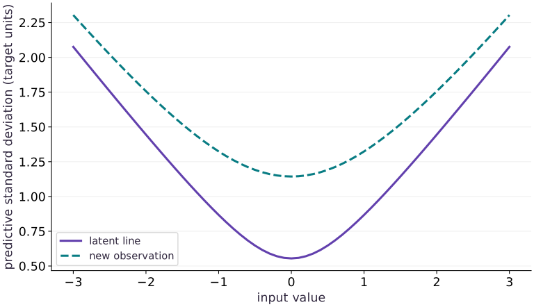
Read the figure

The horizontal axis is the input value. The vertical axis is predictive standard deviation, in target units. The lower curve propagates posterior weight uncertainty; the upper curve also adds the assumed observation noise before taking a square root. At input zero they are about $0.555$ and $1.144$ . The curves rise symmetrically toward both ends because centered training inputs produce zero intercept-slope covariance.

Connect it to the computation

The gap is not a fixed standard deviation of one: variances add, then we take the square root. The lower curve is narrowest near the observed center and grows under extrapolation. These are exact Gaussian-model standard deviations, not measured error bars or empirical coverage on a real test set.

Open full-size figure Download data and provenance

The notebook contains the data experiment, plotting code, and recorded figure output. Rerun it to test your changes.

Where to put & run this code: Work in phases/11-probability/02-build-a-bayesian-regression/code/main.py (or downloaded exercises/probability-02.py / exercises/probability-02.ipynb) and execute from the repository root with python3 phases/11-probability/02-build-a-bayesian-regression/code/main.py.

1 Construct a small linear model

Create a fresh main.py. The first feature is an intercept. Targets contain three deliberately simple synthetic observations; the known noise scale is an assumption.

main.py · append build step 1

# Step 1 — 1. Construct a small linear model: The design has three rows and two columns.
import numpy as np
import jax
import jax.numpy as jnp
X = jnp.array([[1.,-1.],[1.,0.],[1.,1.]])
y = jnp.array([-1.,1.,3.])
sigma, prior_scale = 1., 2.

Code building blocks in this step

jnp.array(values, dtype=...) — Constructs an immutable device-backed JAX array from Python/NumPy values.

The design has three rows and two columns. The weight vector contains intercept then slope.

2 Solve the posterior system

Append the conjugate update. Use a linear solve rather than writing an explicit matrix inverse for the mean.

main.py · append build step 2

# Step 2 — 2. Solve the posterior system: The independent fractions follow because centered inputs make the...
def posterior(X,y,sigma,prior_scale):
    precision = jnp.eye(X.shape[1])/prior_scale**2 + X.T@X/sigma**2
    mean = jnp.linalg.solve(precision,X.T@y/sigma**2)
    covariance = jnp.linalg.solve(precision,jnp.eye(X.shape[1]))
    return mean,covariance
mean,cov = posterior(X,y,sigma,prior_scale)
assert jnp.allclose(mean,jnp.array([12/13,16/9]),atol=1e-6)
assert jnp.allclose(cov,jnp.diag(jnp.array([4/13,4/9])),atol=1e-6)

Code building blocks in this step

jnp.array(values, dtype=...) — Constructs an immutable device-backed JAX array from Python/NumPy values.
jnp.zeros / jnp.ones(shape, dtype=...) — Allocates a tensor of the given shape initialized with constants.
jnp.allclose(actual, expected, rtol=..., atol=...) — Checks that two arrays match elementwise within floating-point tolerance.

The independent fractions follow because centered inputs make the precision matrix diagonal.

3 Predict both the latent mean and a new observation

Append the prediction calculation, then run python main.py. Retain the two variance components separately.

main.py · append build step 3

# Step 3 — 3. Predict both the latent mean and a new observation: The variance at the extrapolation input is larger because slope...
def predictive(design,mean,cov,sigma):
    # Perform matrix / vector contraction (`@`) to compute `center`.
    center = design@mean
    latent_variance = jnp.einsum('ni,ij,nj->n',design,cov,design)
    return center,latent_variance,latent_variance+sigma**2
query = jnp.array([[1.,0.],[1.,2.]])
center,latent_var,observation_var = predictive(query,mean,cov,sigma)
assert jnp.allclose(latent_var,jnp.array([4/13,4/13+16/9]),atol=1e-6)
assert jnp.allclose(observation_var-latent_var,1.)
print('posterior mean:',mean,'covariance:',cov)
print('latent variance:',latent_var,'observation variance:',observation_var)

Code building blocks in this step

jnp.array(values, dtype=...) — Constructs an immutable device-backed JAX array from Python/NumPy values.
jnp.allclose(actual, expected, rtol=..., atol=...) — Checks that two arrays match elementwise within floating-point tolerance.

The variance at the extrapolation input is larger because slope uncertainty contributes more strongly there.

View the cumulative build in main.py

These blocks append in order to the same file.

main.py · cumulative Python build

# Step 1 — 1. Construct a small linear model: The design has three rows and two columns.
import numpy as np
import jax
import jax.numpy as jnp
X = jnp.array([[1.,-1.],[1.,0.],[1.,1.]])
y = jnp.array([-1.,1.,3.])
sigma, prior_scale = 1., 2.

# Step 2 — 2. Solve the posterior system: The independent fractions follow because centered inputs make the...
def posterior(X,y,sigma,prior_scale):
    precision = jnp.eye(X.shape[1])/prior_scale**2 + X.T@X/sigma**2
    mean = jnp.linalg.solve(precision,X.T@y/sigma**2)
    covariance = jnp.linalg.solve(precision,jnp.eye(X.shape[1]))
    return mean,covariance
mean,cov = posterior(X,y,sigma,prior_scale)
assert jnp.allclose(mean,jnp.array([12/13,16/9]),atol=1e-6)
assert jnp.allclose(cov,jnp.diag(jnp.array([4/13,4/9])),atol=1e-6)

# Step 3 — 3. Predict both the latent mean and a new observation: The variance at the extrapolation input is larger because slope...
def predictive(design,mean,cov,sigma):
    # Perform matrix / vector contraction (`@`) to compute `center`.
    center = design@mean
    latent_variance = jnp.einsum('ni,ij,nj->n',design,cov,design)
    return center,latent_variance,latent_variance+sigma**2
query = jnp.array([[1.,0.],[1.,2.]])
center,latent_var,observation_var = predictive(query,mean,cov,sigma)
assert jnp.allclose(latent_var,jnp.array([4/13,4/13+16/9]),atol=1e-6)
assert jnp.allclose(observation_var-latent_var,1.)
print('posterior mean:',mean,'covariance:',cov)
print('latent variance:',latent_var,'observation variance:',observation_var)

Run the example

python3 phases/11-probability/02-build-a-bayesian-regression/code/main.py

About this command

This shortcut uses an activated macOS/Linux course environment in the repository folder. For Windows, use the explicit interpreter command in “Setup help” above. The script includes worked examples and reference solutions.

Inspect the complete assembled example

main.py · complete Python example

# Step 1 — 1. Construct a small linear model: The design has three rows and two columns.
import numpy as np
import jax
import jax.numpy as jnp
X = jnp.array([[1.,-1.],[1.,0.],[1.,1.]])
y = jnp.array([-1.,1.,3.])
sigma, prior_scale = 1., 2.

# Step 2 — 2. Solve the posterior system: The independent fractions follow because centered inputs make the...
def posterior(X,y,sigma,prior_scale):
    precision = jnp.eye(X.shape[1])/prior_scale**2 + X.T@X/sigma**2
    mean = jnp.linalg.solve(precision,X.T@y/sigma**2)
    covariance = jnp.linalg.solve(precision,jnp.eye(X.shape[1]))
    return mean,covariance
mean,cov = posterior(X,y,sigma,prior_scale)
assert jnp.allclose(mean,jnp.array([12/13,16/9]),atol=1e-6)
assert jnp.allclose(cov,jnp.diag(jnp.array([4/13,4/9])),atol=1e-6)

# Step 3 — 3. Predict both the latent mean and a new observation: The variance at the extrapolation input is larger because slope...
def predictive(design,mean,cov,sigma):
    # Perform matrix / vector contraction (`@`) to compute `center`.
    center = design@mean
    latent_variance = jnp.einsum('ni,ij,nj->n',design,cov,design)
    return center,latent_variance,latent_variance+sigma**2
query = jnp.array([[1.,0.],[1.,2.]])
center,latent_var,observation_var = predictive(query,mean,cov,sigma)
assert jnp.allclose(latent_var,jnp.array([4/13,4/13+16/9]),atol=1e-6)
assert jnp.allclose(observation_var-latent_var,1.)
print('posterior mean:',mean,'covariance:',cov)
print('latent variance:',latent_var,'observation variance:',observation_var)

Expected result: The posterior mean is approximately $(0.9231,1.7778)$ . Latent variances at inputs $0,2$ are approximately $0.3077,2.0855$ ; observation variances are each larger by $1$ .

Recorded reference execution

Reference output captured from executing the complete lesson script (code/main.py) and its assertions in the course CPU environment.

2026-10-20T10:48:42.156598+00:00 · Python 3.14.3 · JAX 0.9.2 · 1 CPU device

posterior mean: [0.923077  1.7777778] covariance: [[0.30769232 0.        ]
 [0.         0.44444445]]
latent variance: [0.30769232 2.0854702 ] observation variance: [1.3076923 3.0854702]
posterior mean: [0.923077  1.7777778] covariance: [[0.30769232 0.        ]
 [0.         0.44444445]]
latent variance: [0.30769232 2.0854702 ] observation variance: [1.3076923 3.0854702]
[0.16       0.23529412]
PASS: probability-02

Download execution record · The notebook includes executed cells and figure outputs. Compare your run with these values; timings depend on the machine.

Repeat independent observations

Repeat independent observations · Python experiment

# Experiment — Repeat independent observations: The calculation treats rows as independent new evidence.
repeat_mean,repeat_cov = posterior(jnp.tile(X,(2,1)),jnp.tile(y,2),sigma,prior_scale)
assert jnp.all(jnp.diag(repeat_cov)<jnp.diag(cov))
print(jnp.diag(repeat_cov))

Expected: Both posterior marginal variances decrease.

The calculation treats rows as independent new evidence. Duplicating a stored file does not create new evidence in a real dataset.

Check the prior-only boundary

Check the prior-only boundary · Python experiment

# Experiment — Check the prior-only boundary: The posterior recovers the prior when no likelihood information...
empty_mean,empty_cov = posterior(jnp.empty((0,2)),jnp.empty((0,)),sigma,prior_scale)
assert jnp.allclose(empty_mean,0.)
assert jnp.allclose(empty_cov,4*jnp.eye(2))

Expected: The mean is zero and covariance is $4I$ .

The posterior recovers the prior when no likelihood information is present.

Hands-On Exercise · Modify & Verify Run in the declared lesson environment

Make it yours

Where to put your code: Append your solution at the bottom of phases/11-probability/02-build-a-bayesian-regression/code/main.py (or inside the Make it yours cell of exercises/probability-02.ipynb) and run python3 phases/11-probability/02-build-a-bayesian-regression/code/main.py to verify your prediction before opening the reference solution.

Strengthen the prior by changing its scale from two to one half. Predict the direction of change in the weight norm and check it. Explain why a tighter posterior need not mean a better model.

Show a writing guide and starter scaffold

How to write this exercise code: step-by-step recipe & starter scaffold

1. Key functions & syntax to use:

posterior(...) — Call posterior with your updated parameters or inputs from this lesson's workspace.
linalg.norm(...) — Call linalg.norm with your updated parameters or inputs from this lesson's workspace.
assert condition — Verify that the observed output shape, status, or numerical value satisfies the contract.

2. Step-by-step implementation plan:

Set up the changed input or configuration parameters requested in the prompt.
Run the target function or transformation and assert that the output matches your prediction.

Starter code scaffold · copy into your file & fill in the TODOs

# Exercise solution: Strengthen the prior by changing its scale from two to one half.
strong_mean,strong_cov = posterior(...)  # TODO: compute strong_mean,strong_cov
assert jnp.linalg.norm(strong_mean)  # TODO: complete assertion check
assert jnp.all(jnp.diag(strong_cov)  # TODO: complete assertion check

Reveal the reference solution

Reference solution

# Exercise solution: Strengthen the prior by changing its scale from two to one half.
strong_mean,strong_cov = posterior(X,y,sigma,.5)
assert jnp.linalg.norm(strong_mean)<jnp.linalg.norm(mean)
assert jnp.all(jnp.diag(strong_cov)<jnp.diag(cov))

Move away from centered inputs

Transfer / diagnosis

Use design rows $(1,0),(1,1),(1,2)$ . Compare the JAX result with a host NumPy linear solve and show the posterior covariance is not diagonal.

Show a writing guide and starter scaffold

How to write this practice solution: step-by-step recipe & starter scaffold

1. Key functions & syntax to use:

jnp.array(values, dtype=...) — Constructs an immutable device-backed JAX array from Python/NumPy values.
jnp.allclose(actual, expected, rtol=..., atol=...) — Checks that two arrays match elementwise within floating-point tolerance.

2. Step-by-step implementation plan:

Convert host_X to a host NumPy array for inspection or verification.
Construct an identity matrix host_P.
Convert to a host NumPy array for inspection or verification.

Starter code scaffold · copy into your file & fill in the TODOs

# Move away from centered inputs (Transfer / diagnosis): Nonzero covariance affects prediction uncertainty; keeping...
shift_X = jnp.array(...)  # TODO: compute shift_X
shift_m,shift_c = posterior(...)  # TODO: compute shift_m,shift_c
# Convert `host_X` to a host NumPy array for inspection or verification.
host_X = np.asarray(...)  # TODO: compute host_X
# Construct an identity matrix `host_P`.
host_P = np.eye(...)  # TODO: compute host_P
# Convert `` to a host NumPy array for inspection or verification.
np.testing.assert_allclose(shift_m,np.linalg.solve(host_P,host_X.T@np.asarray(y)),rtol=1e-5,atol=1e-6)
assert shift_c[0,1]  # TODO: complete assertion check

Show a hint

The intercept and slope can compensate for each other when features are not centered.

Reveal reference solution and reasoning

Move away from centered inputs · Python solution

# Move away from centered inputs (Transfer / diagnosis): Nonzero covariance affects prediction uncertainty; keeping...
shift_X = jnp.array([[1.,0.],[1.,1.],[1.,2.]])
shift_m,shift_c = posterior(shift_X,y,sigma,prior_scale)
# Convert `host_X` to a host NumPy array for inspection or verification.
host_X=np.asarray(shift_X,dtype=np.float64)
# Construct an identity matrix `host_P`.
host_P=np.eye(2)/4+host_X.T@host_X
# Convert `` to a host NumPy array for inspection or verification.
np.testing.assert_allclose(shift_m,np.linalg.solve(host_P,host_X.T@np.asarray(y)),rtol=1e-5,atol=1e-6)
assert shift_c[0,1]<0

Nonzero covariance affects prediction uncertainty; keeping only marginal variances would lose the compensating relationship.

Verify total predictive variance

Transfer / diagnosis

Draw posterior weights and independent observation noise. Compare empirical prediction variance at input zero to the analytic observation variance.

Show a writing guide and starter scaffold

How to write this practice solution: step-by-step recipe & starter scaffold

1. Key functions & syntax to use:

jax.random.PRNGKey(seed) & jax.random.split(key) — Manages explicit, stateless PRNG keys—always split a key before passing subkeys into independent random draws.

2. Step-by-step implementation plan:

Create or split explicit PRNG key(s) ((kw, kn)) for reproducible randomness.
Sample deterministic random values into weights using an explicit PRNG key.
Sample deterministic random values into replicated using an explicit PRNG key.

Starter code scaffold · copy into your file & fill in the TODOs

# Verify total predictive variance (Transfer / diagnosis): A simulation verifies that the independent noise term...
# Create or split explicit PRNG key(s) (`(kw, kn)`) for reproducible randomness.
kw,kn = jax.random.split(...)  # TODO: compute kw,kn
# Sample deterministic random values into `weights` using an explicit PRNG key.
weights = ...  # TODO: compute weights
# Sample deterministic random values into `replicated` using an explicit PRNG key.
replicated = ...  # TODO: compute replicated
assert abs(float(replicated.var())-float(observation_var[0]))  # TODO: complete assertion check

Show a hint

Use separate keys for weights and noise; sample with a Cholesky factor.

Reveal reference solution and reasoning

Verify total predictive variance · Python solution

# Verify total predictive variance (Transfer / diagnosis): A simulation verifies that the independent noise term...
# Create or split explicit PRNG key(s) (`(kw, kn)`) for reproducible randomness.
kw,kn=jax.random.split(jax.random.key(37))
# Sample deterministic random values into `weights` using an explicit PRNG key.
weights=mean+jax.random.normal(kw,(30000,2))@jnp.linalg.cholesky(cov).T
# Sample deterministic random values into `replicated` using an explicit PRNG key.
replicated=weights[:,0]+sigma*jax.random.normal(kn,(30000,))
assert abs(float(replicated.var())-float(observation_var[0]))<.07

A simulation verifies that the independent noise term belongs in predictions for observed targets.

Diagnose the result

If an interval becomes implausibly narrow, print the latent and noise variance terms separately. If the slope is unexpectedly shrunk, inspect whether the prior scale was confused with prior precision. If targets have an extra column axis, reject the shape before a matrix operation silently changes the mean shape.

Carry forward

Posterior precision combines prior information with likelihood information.
Latent uncertainty and future observation noise are separate quantities.
An exact small model supplies an independent reference for approximate inference.

Keep your evidence

Download evidence template

Precision derivation, exact fractional reference, host solve and predictive variance plot. Keep the environment, observed outputs and your explanation of the figure.

Save your modified code, its output, and an explanation of your prediction. Checkpoint answers and exercise evidence are tracked separately.

Saved in this browser. Export or back up your portfolio anytime in My learning.

Save work for this lesson

Verified on local CPU. Stage to a Cloud TPU VM via Cloud TPU setup to record accelerator execution receipts (TODO: add automated Cloud TPU CI execution receipts).

Build a Bayesian regression

What you will be able to do

The problem

The idea

Separate uncertainty about the function from observation noise

State what is random

Combine information through precision

Check the special case by hand

Two uncertainty bands answer two questions

Use a tiny exact model as an inference test

Prediction uncertainty grows away from the observed center

Read the figure

Connect it to the computation

1 Construct a small linear model

2 Solve the posterior system

3 Predict both the latent mean and a new observation

Run the example

Recorded reference execution

Repeat independent observations

Check the prior-only boundary

Make it yours

Move away from centered inputs

Verify total predictive variance

Check your understanding

Diagnose the result

Carry forward

Keep your evidence

Primary references