 JAX Pathways
Phase 10 / Scientific computing
Differentiate through a solver
Revision v0.7.0 · Updated since your last visit. Review the changes; your progress is saved.
Lesson · about 105 minutes · CPU practice
Derive an independent discrete solver sensitivity. Check an observation-loss gradient at a nonoptimal parameter.
Phase study guide: preparation, milestones and project evidence
Before you start
Before this: Vectorize trajectories and scan time
Hardware: CPU
Setup help: Python, notebook, or Cloud TPU VM
Use the tested CPU packages (the recorded environment uses Python 3.14.3). Other Python versions and accelerator environments require separate checks. The optional Cloud TPU specialization explains the target-specific execution boundaries. Logical CPU devices practice partitioning; they do not simulate TPU performance.
Download the repository ZIP or use your existing checkout. Extract it and open a terminal in the folder containing requirements-cpu.txt. The beginner ZIP is separate; these lessons use the full repository folder.
python3 -m venv .venv
source .venv/bin/activate
python -m pip install -r requirements-cpu.txtpy -3 -m venv .venv
.\.venv\Scripts\python.exe -m pip install -r requirements-cpu.txtAfter activation, run the complete worked example from that same folder:
python phases/10-science/03-differentiate-through-a-solver/code/main.py.\.venv\Scripts\python.exe phases/10-science/03-differentiate-through-a-solver/code/main.pyFor an incremental build, create main.py in your own practice folder, append each build block in order, and run python main.py with this environment active. Keep that file separate from the downloaded reference solution.
Download this lesson’s notebook. Open it with a Python kernel using the course environment. Run cells from the top after restarting the kernel; experiments depend on earlier definitions.
For local Jupyter, first install the course requirements using the Local Python steps, then use your environment’s Python to start Jupyter:
python -m pip install jupyterlab
python -m jupyter lab.\.venv\Scripts\python.exe -m pip install jupyterlab
.\.venv\Scripts\python.exe -m jupyter labSelect the downloaded science-03.ipynb file in JupyterLab. The notebook contains reference solutions; make your prediction and attempt each practice task before opening them. Restart the kernel before changing logical device setup.
The worked reference for this lesson is CPU-validated. Some references explicitly configure logical CPU devices; setting JAX_PLATFORMS does not adapt them to a TPU. Follow the execution matrix and reviewed multi-host example before attempting a target run.
For accelerator preparation, study TPU setup, observed runtime receipts, checkpointed jobs and precision and retained traces. These target paths remain unqualified on physical TPU hardware until an actual receipt is recorded. Cloud provisioning is optional for CPU learning.
Check: Endpoint autodiff approximately -0.9863878097; continuous reference approximately -0.9863878558. The loss gradient agrees with central differences and decreases the loss when subtracted.
Revisit the guided CPU setup · Open 19: TPU Setup. Package instructions are CPU instructions; Windows and accelerator environments need their own validation.
What you will be able to do
- Derive an independent discrete solver sensitivity.
- Check an observation-loss gradient at a nonoptimal parameter.
- Separate derivative implementation error from discretization error.
- Explain static-grid differentiation and the limits of this solver.
The problem
A simulation can produce a convincing curve and an incorrect sensitivity. Before using gradients to infer a physical parameter, how can we tell whether the derivative is right, and whether it describes the continuous equation closely enough?
The idea
Differentiating a numerical solver gives sensitivity of its discrete computation. That sensitivity can approach the continuous system's sensitivity as the discretization improves, but the two are not automatically identical at a finite step size.
Differentiate the computation you actually executed
For , Euler gives , where is step size and is step count. Differentiating that expression gives . The continuous derivative at time is instead .
These expressions give two distinct references: one checks differentiation through the discrete steps, and the other measures convergence toward the continuous sensitivity. Hold final time fixed as you refine the grid.
In the sensitivity plot, disagreement with the continuous answer can be discretization error even when autodiff is correct. Compare the discrete analytic derivative first, then inspect refinement behavior.
Follow one parameter through every time step
Changing changes every state transition. RK4 on this linear equation is multiplication by , so the final state after steps is . Differentiate that expression with the chain rule. The derivative includes , which is easy to lose when differentiating the polynomial. For our parameters it is about : increasing the rate lowers the remaining temperature.
Check the discrete derivative before asking about physics
JAX and the polynomial derivative agree to near float64 roundoff. The continuous derivative is , approximately at two seconds. Their small difference is expected from the numerical method. A perfect autodiff check cannot remove that bias. Refine the grid and see whether both the state and its sensitivity approach the continuous reference.
Turn a trajectory into a scalar objective
The loss averages squared errors over all forty-one saved times. Its derivative adds each residual multiplied by the sensitivity of that observation, including the factor of two and mean normalization. The initial observation contributes zero rate sensitivity because the initial value is fixed. Evaluate the gradient away from the optimum: at the optimum, both a broken zero gradient and a correct gradient may look similar.
Use a finite-difference window, not one magical epsilon
A central finite difference probes the change in the whole objective. If the perturbation is too large, curvature biases the estimate; if it is too small, subtracting nearly equal floating-point values loses information. Sweep several perturbations and look for a range of agreement. Keep initial state, observations, grid and precision fixed across the comparison. This lesson uses float64; copying its smallest perturbation into a float32 program requires rechecking tolerances.
Know which solver problem you have solved
The grid is fixed and the output length is static. We have not implemented adaptive error control, event handling, stiffness detection or a custom adjoint. A Python integer controls scan length; a parameter-dependent early exit would introduce a different differentiation problem. For richer systems, Diffrax exposes solver choice, tolerances, saved times and adjoint strategies. Its optional extension belongs in a separately pinned and executed environment; these core CPU checks do not validate that library or an adaptive solver.
A solver gradient converges toward the physical sensitivity
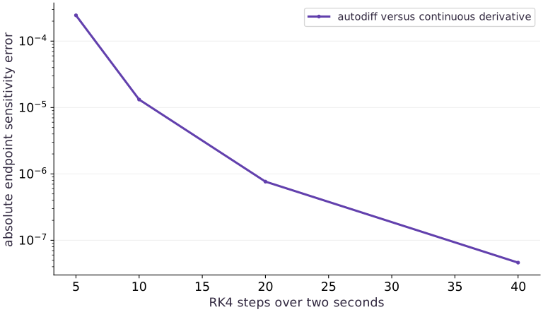
Predict before looking: How much should the gradient error fall when a fourth-order method doubles its steps?
Read the figure
The horizontal axis shows the number of updates over the same two-second horizon. The vertical axis is absolute error in the endpoint derivative with respect to rate, on a logarithmic scale. A lower point means closer agreement with the exact continuous derivative, not a smaller temperature or lower training loss.
With five steps the error is about . At ten, twenty and forty steps it is about , and . The final doubling improves agreement by about , consistent with fourth-order convergence in this range.
Connect it to the computation
The plotted derivatives come from JAX differentiating scan. The reference is the independently derived continuous sensitivity . A separate polynomial check verifies the derivative of the discrete RK4 program to much tighter tolerance.
The downward trend does not prove convergence for a stiff or discontinuous system, and it cannot continue indefinitely at fixed precision. It shows why checking only autodiff against another differentiation of the same program would miss solver bias.
Open full-size figureDownload data and provenance
The notebook contains the data experiment, plotting code, and recorded figure output. Rerun it to test your changes.
Where to put & run this code: Work in phases/10-science/03-differentiate-through-a-solver/code/main.py (or downloaded exercises/science-03.py / exercises/science-03.ipynb) and execute from the repository root with python3 phases/10-science/03-differentiate-through-a-solver/code/main.py.
1 Rebuild the differentiable solver
Append this block to main.py in your CPU course environment; for the first block create the file. Run blocks in order.
# Step 1 — Rebuild the differentiable solver: The solver remains a pure JAX function with a static number of...
import jax
# Update state in place with the new values.
jax.config.update("jax_enable_x64", True)
import jax.numpy as jnp
import numpy as np

def rk4_step(rate, value, dt):
    a = -rate*value
    b = -rate*(value + dt*a/2)
    c = -rate*(value + dt*b/2)
    d = -rate*(value + dt*c)
    return value + dt*(a + 2*b + 2*c + d)/6

# Define `solve(rate, initial, steps, dt)` to carry state across steps with `jax.lax.scan`:
def solve(rate, initial, steps=40, dt=0.05):
    def advance(value, unused):
        next_value = rk4_step(rate, value, dt)
        return next_value, next_value
    # Run compiled structured control flow via `jax.lax` (`(_, tail)`).
    _, tail = jax.lax.scan(advance, initial, None, length=steps)
    return jnp.concatenate((jnp.atleast_1d(initial), tail))
Code building blocks in this step
jax.lax.scan(step_fn, init_carry, xs, length=...)— Compiles a sequential loop wherestep_fn(carry, x)returns(next_carry, y), returning(final_carry, stacked_ys).
The solver remains a pure JAX function with a static number of scan steps. No host conversion occurs inside the differentiated calculation.
2 Check the derivative of the discrete endpoint
Append this block to main.py in your CPU course environment; for the first block create the file. Run blocks in order.
# Step 2 — Check the derivative of the discrete endpoint: Autodiff gives the derivative of the actual RK4 program.
rate, initial, steps, dt = 0.7, jnp.array(2.0), 40, 0.05
endpoint = lambda k: solve(k,initial,steps,dt)[-1]
# Differentiate the objective to obtain `autodiff` via automatic differentiation.
autodiff = float(jax.grad(endpoint)(rate))
z = -rate*dt
r = 1+z+z*z/2+z**3/6+z**4/24
dr_dk = -dt*(1+z+z*z/2+z**3/6)
discrete_gradient = 2.0*steps*r**(steps-1)*dr_dk
continuous_gradient = -2.0*(steps*dt)*np.exp(-rate*steps*dt)
np.testing.assert_allclose(autodiff,discrete_gradient,rtol=1e-11,atol=1e-12)
np.testing.assert_allclose(autodiff,continuous_gradient,rtol=1e-7)
print("Autodiff:",autodiff,"discrete oracle:",discrete_gradient,"continuous oracle:",continuous_gradient)
Code building blocks in this step
jnp.array(values, dtype=...)— Constructs an immutable device-backed JAX array from Python/NumPy values.jnp.allclose(actual, expected, rtol=..., atol=...)— Checks that two arrays match elementwise within floating-point tolerance.jax.grad(loss_fn)(params, ...)— Transforms a scalar-output function into a function returning the gradient PyTree with the same structure asparams.
Autodiff gives the derivative of the actual RK4 program. Compare first against the discrete polynomial derivative, then assess how closely that approximates the continuous sensitivity.
3 Differentiate an observation loss and check its direction
Append this block to main.py in your CPU course environment; for the first block create the file. Run blocks in order.
# Step 3 — Differentiate an observation loss and check its direction: The candidate rate is too large.
times = jnp.arange(steps+1)*dt
observations = 2.0*jnp.exp(-0.7*times)
def objective(k):
    return jnp.mean((solve(k,initial,steps,dt)-observations)**2)
probe = 1.0
# Differentiate the objective to obtain `(value, derivative)` via automatic differentiation.
value, derivative = jax.value_and_grad(objective)(probe)
epsilon = 1e-4
finite_difference = (float(objective(probe+epsilon))-float(objective(probe-epsilon)))/(2*epsilon)
np.testing.assert_allclose(derivative,finite_difference,rtol=2e-7,atol=1e-10)
assert float(derivative) > 0
assert float(objective(probe-0.1*derivative)) < float(value)
print("Loss:",float(value),"gradient:",float(derivative),"finite difference:",finite_difference)
Code building blocks in this step
jnp.arange(n, dtype=...)— Creates a 1-D JAX array of evenly spaced values[0, 1, ..., n-1]on the target device.x.sum(axis=...) / x.mean(axis=..., keepdims=...)— Reduces values along the namedaxis(the axis you name is collapsed unlesskeepdims=True).jnp.allclose(actual, expected, rtol=..., atol=...)— Checks that two arrays match elementwise within floating-point tolerance.jax.value_and_grad(loss_fn)(params, ...)— Evaluates both the scalar loss and its gradient PyTree(loss_val, grads)in a single forward+backward pass.
The candidate rate is too large. Its predictions decay too quickly. A positive loss derivative tells gradient descent to decrease the rate, consistent with that physical diagnosis.
View the cumulative build in main.py
These blocks append in order to the same file.
# Step 1 — Rebuild the differentiable solver: The solver remains a pure JAX function with a static number of...
import jax
# Update state in place with the new values.
jax.config.update("jax_enable_x64", True)
import jax.numpy as jnp
import numpy as np

def rk4_step(rate, value, dt):
    a = -rate*value
    b = -rate*(value + dt*a/2)
    c = -rate*(value + dt*b/2)
    d = -rate*(value + dt*c)
    return value + dt*(a + 2*b + 2*c + d)/6

# Define `solve(rate, initial, steps, dt)` to carry state across steps with `jax.lax.scan`:
def solve(rate, initial, steps=40, dt=0.05):
    def advance(value, unused):
        next_value = rk4_step(rate, value, dt)
        return next_value, next_value
    # Run compiled structured control flow via `jax.lax` (`(_, tail)`).
    _, tail = jax.lax.scan(advance, initial, None, length=steps)
    return jnp.concatenate((jnp.atleast_1d(initial), tail))

# Step 2 — Check the derivative of the discrete endpoint: Autodiff gives the derivative of the actual RK4 program.
rate, initial, steps, dt = 0.7, jnp.array(2.0), 40, 0.05
endpoint = lambda k: solve(k,initial,steps,dt)[-1]
# Differentiate the objective to obtain `autodiff` via automatic differentiation.
autodiff = float(jax.grad(endpoint)(rate))
z = -rate*dt
r = 1+z+z*z/2+z**3/6+z**4/24
dr_dk = -dt*(1+z+z*z/2+z**3/6)
discrete_gradient = 2.0*steps*r**(steps-1)*dr_dk
continuous_gradient = -2.0*(steps*dt)*np.exp(-rate*steps*dt)
np.testing.assert_allclose(autodiff,discrete_gradient,rtol=1e-11,atol=1e-12)
np.testing.assert_allclose(autodiff,continuous_gradient,rtol=1e-7)
print("Autodiff:",autodiff,"discrete oracle:",discrete_gradient,"continuous oracle:",continuous_gradient)

# Step 3 — Differentiate an observation loss and check its direction: The candidate rate is too large.
times = jnp.arange(steps+1)*dt
observations = 2.0*jnp.exp(-0.7*times)
def objective(k):
    return jnp.mean((solve(k,initial,steps,dt)-observations)**2)
probe = 1.0
# Differentiate the objective to obtain `(value, derivative)` via automatic differentiation.
value, derivative = jax.value_and_grad(objective)(probe)
epsilon = 1e-4
finite_difference = (float(objective(probe+epsilon))-float(objective(probe-epsilon)))/(2*epsilon)
np.testing.assert_allclose(derivative,finite_difference,rtol=2e-7,atol=1e-10)
assert float(derivative) > 0
assert float(objective(probe-0.1*derivative)) < float(value)
print("Loss:",float(value),"gradient:",float(derivative),"finite difference:",finite_difference)
Run the example
python3 phases/10-science/03-differentiate-through-a-solver/code/main.pyAbout this command
This shortcut uses an activated macOS/Linux course environment in the repository folder. For Windows, use the explicit interpreter command in “Setup help” above. The script includes worked examples and reference solutions.
Inspect the complete assembled example
# Step 1 — Rebuild the differentiable solver: The solver remains a pure JAX function with a static number of...
import jax
# Update state in place with the new values.
jax.config.update("jax_enable_x64", True)
import jax.numpy as jnp
import numpy as np

def rk4_step(rate, value, dt):
    a = -rate*value
    b = -rate*(value + dt*a/2)
    c = -rate*(value + dt*b/2)
    d = -rate*(value + dt*c)
    return value + dt*(a + 2*b + 2*c + d)/6

# Define `solve(rate, initial, steps, dt)` to carry state across steps with `jax.lax.scan`:
def solve(rate, initial, steps=40, dt=0.05):
    def advance(value, unused):
        next_value = rk4_step(rate, value, dt)
        return next_value, next_value
    # Run compiled structured control flow via `jax.lax` (`(_, tail)`).
    _, tail = jax.lax.scan(advance, initial, None, length=steps)
    return jnp.concatenate((jnp.atleast_1d(initial), tail))

# Step 2 — Check the derivative of the discrete endpoint: Autodiff gives the derivative of the actual RK4 program.
rate, initial, steps, dt = 0.7, jnp.array(2.0), 40, 0.05
endpoint = lambda k: solve(k,initial,steps,dt)[-1]
# Differentiate the objective to obtain `autodiff` via automatic differentiation.
autodiff = float(jax.grad(endpoint)(rate))
z = -rate*dt
r = 1+z+z*z/2+z**3/6+z**4/24
dr_dk = -dt*(1+z+z*z/2+z**3/6)
discrete_gradient = 2.0*steps*r**(steps-1)*dr_dk
continuous_gradient = -2.0*(steps*dt)*np.exp(-rate*steps*dt)
np.testing.assert_allclose(autodiff,discrete_gradient,rtol=1e-11,atol=1e-12)
np.testing.assert_allclose(autodiff,continuous_gradient,rtol=1e-7)
print("Autodiff:",autodiff,"discrete oracle:",discrete_gradient,"continuous oracle:",continuous_gradient)

# Step 3 — Differentiate an observation loss and check its direction: The candidate rate is too large.
times = jnp.arange(steps+1)*dt
observations = 2.0*jnp.exp(-0.7*times)
def objective(k):
    return jnp.mean((solve(k,initial,steps,dt)-observations)**2)
probe = 1.0
# Differentiate the objective to obtain `(value, derivative)` via automatic differentiation.
value, derivative = jax.value_and_grad(objective)(probe)
epsilon = 1e-4
finite_difference = (float(objective(probe+epsilon))-float(objective(probe-epsilon)))/(2*epsilon)
np.testing.assert_allclose(derivative,finite_difference,rtol=2e-7,atol=1e-10)
assert float(derivative) > 0
assert float(objective(probe-0.1*derivative)) < float(value)
print("Loss:",float(value),"gradient:",float(derivative),"finite difference:",finite_difference)
Expected result: Endpoint autodiff approximately -0.9863878097; continuous reference approximately -0.9863878558. The loss gradient agrees with central differences and decreases the loss when subtracted.
Recorded reference execution
Reference output captured from executing the complete lesson script (code/main.py) and its assertions in the course CPU environment.
Autodiff: -0.9863878096749447 discrete oracle: -0.9863878096749429 continuous oracle: -0.9863878557664257
Loss: 0.04837454286198381 gradient: 0.2686922266772409 finite difference: 0.26869222316237146
Autodiff: -0.9863878096749447 discrete oracle: -0.9863878096749429 continuous oracle: -0.9863878557664257
Loss: 0.04837454286198381 gradient: 0.2686922266772409 finite difference: 0.26869222316237146
Sensitivity errors: [np.float64(0.0002448795513753099), np.float64(1.3192617195456613e-05), np.float64(7.654351459329689e-07), np.float64(4.6091481076260266e-08)]
Finite-difference absolute errors: [3.515348206362123e-05, 3.5151551858181307e-07, 3.514869451048952e-09, 3.5118241648035564e-11, 1.1179057679555626e-11]
Rate and initial-state sensitivities: -2.695973769291141 0.44932896460456245
Weighted derivative reference: 0.30367311533053687
Detached autodiff is zero; actual value sensitivity: 0.26869222316237146
PASS: science-03
Download execution record · The notebook includes executed cells and figure outputs. Compare your run with these values; timings depend on the machine.
Watch derivative discretization error shrink
# Experiment — Watch derivative discretization error shrink: Fourth-order convergence becomes visible as an error ratio near...
step_counts = np.array([5,10,20,40])
gradient_errors = []
for n in step_counts:
    # Differentiate the objective to obtain `numerical` via automatic differentiation.
    numerical = jax.grad(lambda k: solve(k,jnp.array(2.0),int(n),2.0/int(n))[-1])(0.7)
    gradient_errors.append(abs(float(numerical)-continuous_gradient))
assert np.all(np.diff(gradient_errors) < 0)
assert 12 < gradient_errors[-2]/gradient_errors[-1] < 20
print("Sensitivity errors:",gradient_errors)
Expected: Errors approximately [2.449e-4, 1.319e-5, 7.654e-7, 4.609e-8].
Fourth-order convergence becomes visible as an error ratio near sixteen when the step is halved. Roundoff will eventually limit this trend.
Sweep central-difference perturbations
# Experiment — Sweep central-difference perturbations: Use the measured errors to select a tolerance.
epsilons = [1e-2,1e-3,1e-4,1e-5,1e-6]
fd_errors=[]
for eps in epsilons:
    fd=(float(objective(probe+eps))-float(objective(probe-eps)))/(2*eps)
    fd_errors.append(abs(fd-float(derivative)))
assert min(fd_errors) < 1e-8
print("Finite-difference absolute errors:",fd_errors)
Expected: There is a useful agreement window; very small perturbations eventually encounter subtraction error.
Use the measured errors to select a tolerance. Do not require every epsilon to improve monotonically.
Make it yours
Where to put your code: Append your solution at the bottom of phases/10-science/03-differentiate-through-a-solver/code/main.py (or inside the Make it yours cell of exercises/science-03.ipynb) and run python3 phases/10-science/03-differentiate-through-a-solver/code/main.py to verify your prediction before opening the reference solution.
Change the initial value to and the rate to . Verify the endpoint gradient against the continuous derivative, then check the derivative with respect to the initial value as well.
Show a writing guide and starter scaffold
How to write this exercise code: step-by-step recipe & starter scaffold
1. Key functions & syntax to use:
jnp.array(values, dtype=...)— Constructs an immutable device-backed JAX array from Python/NumPy values.jnp.allclose(actual, expected, rtol=..., atol=...)— Checks that two arrays match elementwise within floating-point tolerance.jax.grad(loss_fn)(params, ...)— Transforms a scalar-output function into a function returning the gradient PyTree with the same structure asparams.
2. Step-by-step implementation plan:
- Differentiate the objective to obtain
g_ratevia automatic differentiation. - Differentiate the objective to obtain
g_initialvia automatic differentiation.
# Exercise solution: Change the initial value to 3 and the rate to 0.4.
changed_rate, changed_initial = ...  # TODO: compute changed_rate, changed_initial
# Differentiate the objective to obtain `g_rate` via automatic differentiation.
g_rate = jax.grad(...)  # TODO: compute g_rate
# Differentiate the objective to obtain `g_initial` via automatic differentiation.
g_initial = jax.grad(...)  # TODO: compute g_initial
np.testing.assert_allclose(g_rate,-2*changed_initial*np.exp(-0.8),rtol=1e-7)
np.testing.assert_allclose(g_initial,np.exp(-0.8),rtol=1e-8)
print("Rate and initial-state sensitivities:",float(g_rate),float(g_initial))
Reveal the reference solution
# Exercise solution: Change the initial value to 3 and the rate to 0.4.
changed_rate, changed_initial = 0.4, 3.0
# Differentiate the objective to obtain `g_rate` via automatic differentiation.
g_rate = jax.grad(lambda k: solve(k,jnp.array(changed_initial))[-1])(changed_rate)
# Differentiate the objective to obtain `g_initial` via automatic differentiation.
g_initial = jax.grad(lambda u: solve(changed_rate,u)[-1])(changed_initial)
np.testing.assert_allclose(g_rate,-2*changed_initial*np.exp(-0.8),rtol=1e-7)
np.testing.assert_allclose(g_initial,np.exp(-0.8),rtol=1e-8)
print("Rate and initial-state sensitivities:",float(g_rate),float(g_initial))
Weight observations without losing normalization
Practice
Differentiate a weighted observation loss that emphasizes late times. Compare with a NumPy chain-rule reference built from the RK4 polynomial.
Show a writing guide and starter scaffold
How to write this practice solution: step-by-step recipe & starter scaffold
1. Key functions & syntax to use:
jnp.array(values, dtype=...)— Constructs an immutable device-backed JAX array from Python/NumPy values.x.sum(axis=...) / x.mean(axis=..., keepdims=...)— Reduces values along the namedaxis(the axis you name is collapsed unlesskeepdims=True).jnp.allclose(actual, expected, rtol=..., atol=...)— Checks that two arrays match elementwise within floating-point tolerance.jax.grad(loss_fn)(params, ...)— Transforms a scalar-output function into a function returning the gradient PyTree with the same structure asparams.
2. Step-by-step implementation plan:
- Aggregate array values to compute
reference. - Differentiate the objective to obtain gradients
.
# Weight observations without losing normalization (Practice): The independent expression checks reduction normalization...
weights = np.linspace(...)  # TODO: compute weights
def weighted_objective(k):
    residual = solve(...)  # TODO: compute residual
    return ...  # TODO: return computed result
k = ...  # TODO: compute k
h = ...  # TODO: compute h
n = np.arange(...)  # TODO: compute n
z = ...  # TODO: compute z
r = ...  # TODO: compute r
dr = ...  # TODO: compute dr
u = ...  # TODO: compute u
sensitivity = ...  # TODO: compute sensitivity
# Aggregate array values to compute `reference`.
reference = np.sum(...)  # TODO: compute reference
# Differentiate the objective to obtain gradients ``.
np.testing.assert_allclose(jax.grad(weighted_objective)(k),reference,rtol = ...  # TODO: compute np.testing.assert_allclose(jax.grad(weighted_objective)(k),reference,rtol
print("Weighted derivative reference:",reference)
Show a hint
Weights change the observation importance and must be normalized explicitly.
Reveal reference solution and reasoning
# Weight observations without losing normalization (Practice): The independent expression checks reduction normalization...
weights=np.linspace(0.2,2.0,41)
def weighted_objective(k):
    residual=solve(k,jnp.array(2.0))-observations
    return jnp.sum(jnp.asarray(weights)*residual**2)/np.sum(weights)
k=1.0
h=0.05
n=np.arange(41)
z=-k*h
r=1+z+z*z/2+z**3/6+z**4/24
dr=-h*(1+z+z*z/2+z**3/6)
u=2*r**n
sensitivity=2*n*r**np.maximum(n-1,0)*dr
# Aggregate array values to compute `reference`.
reference=np.sum(2*weights*(u-np.asarray(observations))*sensitivity)/weights.sum()
# Differentiate the objective to obtain gradients ``.
np.testing.assert_allclose(jax.grad(weighted_objective)(k),reference,rtol=1e-11,atol=1e-12)
print("Weighted derivative reference:",reference)
The independent expression checks reduction normalization and the derivative at every saved time, rather than only the endpoint.
Diagnose a detached backward path
Challenge
Reproduce an accidentally detached simulation and explain why a finite-difference test catches it.
Show a writing guide and starter scaffold
How to write this practice solution: step-by-step recipe & starter scaffold
1. Key functions & syntax to use:
jnp.array(values, dtype=...)— Constructs an immutable device-backed JAX array from Python/NumPy values.x.sum(axis=...) / x.mean(axis=..., keepdims=...)— Reduces values along the namedaxis(the axis you name is collapsed unlesskeepdims=True).jax.grad(loss_fn)(params, ...)— Transforms a scalar-output function into a function returning the gradient PyTree with the same structure asparams.
2. Step-by-step implementation plan:
- Define
detached_objective(k)to evaluate the objective and its automatic derivatives:
# Diagnose a detached backward path (Challenge): A plausible forward curve does not validate backward behavior.
# Define `detached_objective(k)` to evaluate the objective and its automatic derivatives:
def detached_objective(k):
    prediction = jax.lax.stop_gradient(...)  # TODO: compute prediction
    return ...  # TODO: return computed result
assert float(jax.grad(detached_objective)(1.0))  # TODO: complete assertion check
fd = ...  # TODO: compute fd
assert abs(fd)  # TODO: complete assertion check
print("Detached autodiff is zero; actual value sensitivity:",fd)
Show a hint
stop_gradient preserves values but removes their derivative.
Reveal reference solution and reasoning
# Diagnose a detached backward path (Challenge): A plausible forward curve does not validate backward behavior.
# Define `detached_objective(k)` to evaluate the objective and its automatic derivatives:
def detached_objective(k):
    prediction=jax.lax.stop_gradient(solve(k,jnp.array(2.0)))
    return jnp.mean((prediction-observations)**2)
assert float(jax.grad(detached_objective)(1.0)) == 0.0
fd=(float(detached_objective(1.0001))-float(detached_objective(0.9999)))/0.0002
assert abs(fd)>1e-3
print("Detached autodiff is zero; actual value sensitivity:",fd)
A plausible forward curve does not validate backward behavior. Remove an unintended gradient barrier and repeat the independent check.
Diagnose the result
If the analytic continuous derivative differs from autodiff, first compare with the discrete polynomial derivative. If only the continuous comparison fails, refine the grid. If a finite difference is nonzero but autodiff is zero, inspect stop_gradient or host conversions. If changing the step count also changes the horizon, repair the experiment before interpreting convergence.
Carry forward
- Follow one parameter through every time step
- Check the discrete derivative before asking about physics
- Turn a trajectory into a scalar objective
- Use a finite-difference window, not one magical epsilon
- Know which solver problem you have solved
Keep your evidence
Polynomial derivative, finite-difference window, sensitivity refinement and detached-gradient diagnosis. Keep the environment, observed outputs and your explanation of the figure.
Save your modified code, its output, and an explanation of your prediction. Checkpoint answers and exercise evidence are tracked separately.
Saved in this browser. Export or back up your portfolio anytime in My learning.
Verified on local CPU. Stage to a Cloud TPU VM via Cloud TPU setup to record accelerator execution receipts (TODO: add automated Cloud TPU CI execution receipts).