 JAX Pathways
Phase 10 / Scientific computing
Fit parameters and scale the simulation
Revision v0.7.0 · Updated since your last visit. Review the changes; your progress is saved.
Lesson · about 115 minutes · CPU practice
Fit a constrained physical parameter through an executed simulator. Separate training fit, held-out prediction and solver refinement.
Phase study guide: preparation, milestones and project evidence
Before you start
Before this: Differentiate through a solver
Hardware: CPU
Setup help: Python, notebook, or Cloud TPU VM
Use the tested CPU packages (the recorded environment uses Python 3.14.3). Other Python versions and accelerator environments require separate checks. The optional Cloud TPU specialization explains the target-specific execution boundaries. Logical CPU devices practice partitioning; they do not simulate TPU performance.
Download the repository ZIP or use your existing checkout. Extract it and open a terminal in the folder containing requirements-cpu.txt. The beginner ZIP is separate; these lessons use the full repository folder.
python3 -m venv .venv
source .venv/bin/activate
python -m pip install -r requirements-cpu.txtpy -3 -m venv .venv
.\.venv\Scripts\python.exe -m pip install -r requirements-cpu.txtAfter activation, run the complete worked example from that same folder:
python phases/10-science/04-fit-parameters-and-scale-the-simulation/code/main.py.\.venv\Scripts\python.exe phases/10-science/04-fit-parameters-and-scale-the-simulation/code/main.pyFor an incremental build, create main.py in your own practice folder, append each build block in order, and run python main.py with this environment active. Keep that file separate from the downloaded reference solution.
Download this lesson’s notebook. Open it with a Python kernel using the course environment. Run cells from the top after restarting the kernel; experiments depend on earlier definitions.
For local Jupyter, first install the course requirements using the Local Python steps, then use your environment’s Python to start Jupyter:
python -m pip install jupyterlab
python -m jupyter lab.\.venv\Scripts\python.exe -m pip install jupyterlab
.\.venv\Scripts\python.exe -m jupyter labSelect the downloaded science-04.ipynb file in JupyterLab. The notebook contains reference solutions; make your prediction and attempt each practice task before opening them. Restart the kernel before changing logical device setup.
The worked reference for this lesson is CPU-validated. Some references explicitly configure logical CPU devices; setting JAX_PLATFORMS does not adapt them to a TPU. Follow the execution matrix and reviewed multi-host example before attempting a target run.
For accelerator preparation, study TPU setup, observed runtime receipts, checkpointed jobs and precision and retained traces. These target paths remain unqualified on physical TPU hardware until an actual receipt is recorded. Cloud provisioning is optional for CPU learning.
Check: The rate moves from 1.4 to approximately 0.700000009. Held-out and refined-grid RMSE stay below 1e-7; initial-only observations have zero rate gradient.
Revisit the guided CPU setup · Open 19: TPU Setup. Package instructions are CPU instructions; Windows and accelerator environments need their own validation.
What you will be able to do
- Fit a constrained physical parameter through an executed simulator.
- Separate training fit, held-out prediction and solver refinement.
- Diagnose unidentifiable observations and discretization-induced parameter bias.
- Measure synchronized batched CPU execution without claiming accelerator scaling.
The problem
Suppose we can observe cooling trajectories but do not know the rate. Can we recover it without confusing optimizer success with a trustworthy physical inference? We will fit a positive rate, test new initial conditions, examine non-identifiability, and measure a batched CPU workload with explicit timing boundaries.
The idea
An inverse problem uses observations to infer parameters of a forward model. A small fitting error is meaningful only if the observations contain information about those parameters and the forward model matches the observation process.
Ask whether observations identify the parameter
For exponential decay , an observation only at equals for every rate . No optimizer can recover the rate from that observation alone. Later observations supply rate information, provided their noise and timing are understood.
The fitting loop changes the parameter, runs the solver at the declared observation times and compares with the data. Keep those times fixed when comparing candidate parameters. Solver error can otherwise be mistaken for a physical parameter effect.
Read the fitted trajectory alongside the residuals and objective history. A decreasing objective shows progress on that objective; it is separate from uniqueness or uncertainty. Test a changed observation schedule to see which part of the result is supported by data.
Choose data that can reveal the parameter
We generate observations from the exponential at forty-one times for initial values , and . The analytic generator is independent of RK4, avoiding a perfect fit caused merely by using exactly the same numerical algorithm twice. The data are noiseless and synthetic. Their provenance and split must remain explicit in any report.
Enforce positivity through a parameterization
An unconstrained update to could make the cooling rate negative, turning decay into growth. Instead train . The chain rule gives ; this changes the optimization geometry as well as enforcing positivity. We start at , twice the true value, and use an explicit fixed learning rate. No claim is made that this rate is suitable for other units or systems.
Inspect the recovered model beyond the training curve
The recovered rate is about , close to the known . The tiny difference is numerical: RK4 slightly approximates the exponential. We test new initial conditions , and , then halve the simulation step. A fitted parameter that changes materially under grid refinement may be compensating for solver error. Good held-out performance here tests the same equation on new starts; it is separate from generalization to a different physical law. On this noiseless fixture, the fitted rate compensates for the tiny RK4 bias: the original-grid held-out error is near roundoff, while finer-grid error is about . Refinement can therefore increase this already tiny residual. The check requires a small error, not automatic improvement.
Recognize observations that cannot identify a parameter
At time zero the state equals the prescribed initial condition regardless of the rate. If the dataset contains only initial observations, the loss gradient is zero for every rate and no optimizer can recover it. This is non-identifiability, not a learning-rate problem. With noisy data, late-time points may also carry little useful signal after the system has nearly decayed. Inspect sensitivities and measurement precision before collecting more equally uninformative data.
Keep numerical bias separate from physical estimates
For an Euler step, matching an exact exponential interval means . Thus a coarse Euler fit can perfectly match these observations using the wrong physical rate. With , a true rate of looks like about . Low training error is not enough to justify the inferred parameter.
Measure a bounded scaling experiment
Compile and warm up each batch shape, place its inputs before the timed region, and wait for results with block_until_ready. Report both total milliseconds and time per trajectory. Changing batch shape may compile a new program. This CPU experiment measures a fixed forty-step output-producing solve; it does not measure training, input transfer, multi-host communication or TPU performance. A batch can amortize overhead without implying unlimited scaling.
Move from this audit to a scientific workflow
The staged scientific-inverse project asks for a reusable simulation and fitting API with changed parameters, noisy observations, held-out checks and a reproducible report. For stiff or adaptive models, choose and validate a suitable solver before reusing the optimizer. Diffrax, Equinox and Lineax provide ecosystem building blocks, but this phase’s executed core intentionally uses the installed JAX environment; no optional library or target hardware execution is implied.
Recover a physical rate, then check what the fit means
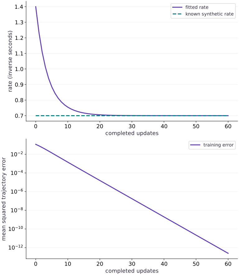
Predict before looking: Does a falling loss alone prove that the recovered rate is physically correct?
Read the figure
The top panel shows the positive rate estimate versus completed optimizer updates. Update is the initial , before training. The reference line is the known synthetic rate . By update , the fitted rate is about ; by update , about .
The lower panel shows mean squared trajectory error on a logarithmic scale. Its initial value is about , falling to about after twenty updates. The displayed first sixty updates focus on the informative descent rather than the eventual floating-point floor.
Connect it to the computation
These recorded post-update values correspond to the same parameters shown above. The reference observations come from the analytic exponential, while fitting uses RK4, so agreement tests a numerical model against independently generated data.
A tiny final loss is plausible for noiseless synthetic data and a single smooth parameter. It is not an uncertainty estimate or proof about real instruments. Held-out starts, grid refinement and the deliberately biased Euler example provide the additional evidence needed to interpret the parameter.
Open full-size figureDownload data and provenance
The notebook contains the data experiment, plotting code, and recorded figure output. Rerun it to test your changes.
Where to put & run this code: Work in phases/10-science/04-fit-parameters-and-scale-the-simulation/code/main.py (or downloaded exercises/science-04.py / exercises/science-04.ipynb) and execute from the repository root with python3 phases/10-science/04-fit-parameters-and-scale-the-simulation/code/main.py.
1 Define the simulator and immutable observations
Append this block to main.py in your CPU course environment; for the first block create the file. Run blocks in order.
# Step 1 — Define the simulator and immutable observations: Observations come from the analytic physical model, not the same...
import jax
# Update state in place with the new values.
jax.config.update("jax_enable_x64", True)
import jax.numpy as jnp
import numpy as np

def rk4_step(rate, value, dt):
    a = -rate*value
    b = -rate*(value + dt*a/2)
    c = -rate*(value + dt*b/2)
    d = -rate*(value + dt*c)
    return value + dt*(a + 2*b + 2*c + d)/6

# Define `solve(rate, initial, steps, dt)` to carry state across steps with `jax.lax.scan`:
def solve(rate, initial, steps=40, dt=0.05):
    def advance(value, unused):
        next_value = rk4_step(rate, value, dt)
        return next_value, next_value
    # Run compiled structured control flow via `jax.lax` (`(_, tail)`).
    _, tail = jax.lax.scan(advance, initial, None, length=steps)
    return jnp.concatenate((jnp.atleast_1d(initial), tail))

train_initials = jnp.array([0.7,1.5,2.3])
times = jnp.arange(41)*0.05
true_rate = 0.7
observations = train_initials[:,None]*jnp.exp(-true_rate*times)
def predict(rate, initials):
    return jax.vmap(lambda initial: solve(rate,initial))(initials)
def objective(log_rate):
    residual = predict(jnp.exp(log_rate),train_initials)-observations
    return jnp.mean(residual**2)
Code building blocks in this step
jnp.arange(n, dtype=...)— Creates a 1-D JAX array of evenly spaced values[0, 1, ..., n-1]on the target device.jnp.array(values, dtype=...)— Constructs an immutable device-backed JAX array from Python/NumPy values.x.sum(axis=...) / x.mean(axis=..., keepdims=...)— Reduces values along the namedaxis(the axis you name is collapsed unlesskeepdims=True).jax.vmap(fn, in_axes=..., out_axes=...)— Vectorizes a single-example function across a batch axis without writing a Python loop.
Observations come from the analytic physical model, not the same discrete solver used for fitting. Different initial values are reserved for evaluation.
2 Fit a positive rate with an explicit update
Append this block to main.py in your CPU course environment; for the first block create the file. Run blocks in order.
# Step 2 — Fit a positive rate with an explicit update: The logarithm parameterization keeps the rate positive.
# Define and JIT-compile `update(log_rate)` so XLA traces and fuses the operations:
@jax.jit
def update(log_rate):
    return log_rate - 0.4*jax.grad(objective)(log_rate)
log_rate = jnp.log(1.4)
loss_history = [float(objective(log_rate))]
rate_history = [float(jnp.exp(log_rate))]
for _ in range(160):
    log_rate = update(log_rate)
    loss_history.append(float(objective(log_rate)))
    rate_history.append(float(jnp.exp(log_rate)))
fitted_rate = float(jnp.exp(log_rate))
assert abs(fitted_rate-true_rate) < 2e-7
assert loss_history[-1] < 1e-20
print("Initial/fitted rate:",rate_history[0],fitted_rate)
print("Initial/final loss:",loss_history[0],loss_history[-1])
Code building blocks in this step
jax.grad(loss_fn)(params, ...)— Transforms a scalar-output function into a function returning the gradient PyTree with the same structure asparams.jax.jit(fn) / @jax.jit— Tracesfnwith abstract shapes and compiles a fused XLA executable cached by input shape and dtype.
The logarithm parameterization keeps the rate positive. The recorded first point is before any update; every later point evaluates the updated parameter.
3 Validate on unseen initial conditions and a finer grid
Append this block to main.py in your CPU course environment; for the first block create the file. Run blocks in order.
# Step 3 — Validate on unseen initial conditions and a finer grid: Held-out starts test transfer within this known equation.
held_initials=jnp.array([0.4,1.1,3.2])
# Convert `held_truth` to a host NumPy array for inspection or verification.
held_truth=np.asarray(held_initials)[:,None]*np.exp(-true_rate*np.asarray(times))
# Convert `held_prediction` to a host NumPy array for inspection or verification.
held_prediction=np.asarray(predict(fitted_rate,held_initials))
# Aggregate array values to compute `held_rmse`.
held_rmse=float(np.sqrt(np.mean((held_prediction-held_truth)**2)))
assert held_rmse < 1e-7
# Vectorize across the batch dimension with `jax.vmap` (`fine`).
fine=np.asarray(jax.vmap(lambda initial:solve(fitted_rate,initial,80,0.025))(held_initials))[:,::2]
# Aggregate array values to compute `fine_rmse`.
fine_rmse=float(np.sqrt(np.mean((fine-held_truth)**2)))
assert fine_rmse < 1e-7
# Differentiate the objective to obtain `initial_only_gradient` via automatic differentiation.
initial_only_gradient=jax.grad(lambda p:jnp.mean((predict(jnp.exp(p),train_initials)[:,0]-observations[:,0])**2))(jnp.log(1.4))
assert float(initial_only_gradient)==0.0
print("Held-out RMSE:",held_rmse,"finer-grid RMSE:",fine_rmse)
print("Initial-time-only gradient:",float(initial_only_gradient))
Code building blocks in this step
jnp.array(values, dtype=...)— Constructs an immutable device-backed JAX array from Python/NumPy values.x.sum(axis=...) / x.mean(axis=..., keepdims=...)— Reduces values along the namedaxis(the axis you name is collapsed unlesskeepdims=True).jax.grad(loss_fn)(params, ...)— Transforms a scalar-output function into a function returning the gradient PyTree with the same structure asparams.jax.vmap(fn, in_axes=..., out_axes=...)— Vectorizes a single-example function across a batch axis without writing a Python loop.
Held-out starts test transfer within this known equation. Refinement tests whether fitting exploited numerical bias. Initial-time-only data cannot identify the decay rate at all.
View the cumulative build in main.py
These blocks append in order to the same file.
# Step 1 — Define the simulator and immutable observations: Observations come from the analytic physical model, not the same...
import jax
# Update state in place with the new values.
jax.config.update("jax_enable_x64", True)
import jax.numpy as jnp
import numpy as np

def rk4_step(rate, value, dt):
    a = -rate*value
    b = -rate*(value + dt*a/2)
    c = -rate*(value + dt*b/2)
    d = -rate*(value + dt*c)
    return value + dt*(a + 2*b + 2*c + d)/6

# Define `solve(rate, initial, steps, dt)` to carry state across steps with `jax.lax.scan`:
def solve(rate, initial, steps=40, dt=0.05):
    def advance(value, unused):
        next_value = rk4_step(rate, value, dt)
        return next_value, next_value
    # Run compiled structured control flow via `jax.lax` (`(_, tail)`).
    _, tail = jax.lax.scan(advance, initial, None, length=steps)
    return jnp.concatenate((jnp.atleast_1d(initial), tail))

train_initials = jnp.array([0.7,1.5,2.3])
times = jnp.arange(41)*0.05
true_rate = 0.7
observations = train_initials[:,None]*jnp.exp(-true_rate*times)
def predict(rate, initials):
    return jax.vmap(lambda initial: solve(rate,initial))(initials)
def objective(log_rate):
    residual = predict(jnp.exp(log_rate),train_initials)-observations
    return jnp.mean(residual**2)

# Step 2 — Fit a positive rate with an explicit update: The logarithm parameterization keeps the rate positive.
# Define and JIT-compile `update(log_rate)` so XLA traces and fuses the operations:
@jax.jit
def update(log_rate):
    return log_rate - 0.4*jax.grad(objective)(log_rate)
log_rate = jnp.log(1.4)
loss_history = [float(objective(log_rate))]
rate_history = [float(jnp.exp(log_rate))]
for _ in range(160):
    log_rate = update(log_rate)
    loss_history.append(float(objective(log_rate)))
    rate_history.append(float(jnp.exp(log_rate)))
fitted_rate = float(jnp.exp(log_rate))
assert abs(fitted_rate-true_rate) < 2e-7
assert loss_history[-1] < 1e-20
print("Initial/fitted rate:",rate_history[0],fitted_rate)
print("Initial/final loss:",loss_history[0],loss_history[-1])

# Step 3 — Validate on unseen initial conditions and a finer grid: Held-out starts test transfer within this known equation.
held_initials=jnp.array([0.4,1.1,3.2])
# Convert `held_truth` to a host NumPy array for inspection or verification.
held_truth=np.asarray(held_initials)[:,None]*np.exp(-true_rate*np.asarray(times))
# Convert `held_prediction` to a host NumPy array for inspection or verification.
held_prediction=np.asarray(predict(fitted_rate,held_initials))
# Aggregate array values to compute `held_rmse`.
held_rmse=float(np.sqrt(np.mean((held_prediction-held_truth)**2)))
assert held_rmse < 1e-7
# Vectorize across the batch dimension with `jax.vmap` (`fine`).
fine=np.asarray(jax.vmap(lambda initial:solve(fitted_rate,initial,80,0.025))(held_initials))[:,::2]
# Aggregate array values to compute `fine_rmse`.
fine_rmse=float(np.sqrt(np.mean((fine-held_truth)**2)))
assert fine_rmse < 1e-7
# Differentiate the objective to obtain `initial_only_gradient` via automatic differentiation.
initial_only_gradient=jax.grad(lambda p:jnp.mean((predict(jnp.exp(p),train_initials)[:,0]-observations[:,0])**2))(jnp.log(1.4))
assert float(initial_only_gradient)==0.0
print("Held-out RMSE:",held_rmse,"finer-grid RMSE:",fine_rmse)
print("Initial-time-only gradient:",float(initial_only_gradient))
Run the example
python3 phases/10-science/04-fit-parameters-and-scale-the-simulation/code/main.pyAbout this command
This shortcut uses an activated macOS/Linux course environment in the repository folder. For Windows, use the explicit interpreter command in “Setup help” above. The script includes worked examples and reference solutions.
Inspect the complete assembled example
# Step 1 — Define the simulator and immutable observations: Observations come from the analytic physical model, not the same...
import jax
# Update state in place with the new values.
jax.config.update("jax_enable_x64", True)
import jax.numpy as jnp
import numpy as np

def rk4_step(rate, value, dt):
    a = -rate*value
    b = -rate*(value + dt*a/2)
    c = -rate*(value + dt*b/2)
    d = -rate*(value + dt*c)
    return value + dt*(a + 2*b + 2*c + d)/6

# Define `solve(rate, initial, steps, dt)` to carry state across steps with `jax.lax.scan`:
def solve(rate, initial, steps=40, dt=0.05):
    def advance(value, unused):
        next_value = rk4_step(rate, value, dt)
        return next_value, next_value
    # Run compiled structured control flow via `jax.lax` (`(_, tail)`).
    _, tail = jax.lax.scan(advance, initial, None, length=steps)
    return jnp.concatenate((jnp.atleast_1d(initial), tail))

train_initials = jnp.array([0.7,1.5,2.3])
times = jnp.arange(41)*0.05
true_rate = 0.7
observations = train_initials[:,None]*jnp.exp(-true_rate*times)
def predict(rate, initials):
    return jax.vmap(lambda initial: solve(rate,initial))(initials)
def objective(log_rate):
    residual = predict(jnp.exp(log_rate),train_initials)-observations
    return jnp.mean(residual**2)

# Step 2 — Fit a positive rate with an explicit update: The logarithm parameterization keeps the rate positive.
# Define and JIT-compile `update(log_rate)` so XLA traces and fuses the operations:
@jax.jit
def update(log_rate):
    return log_rate - 0.4*jax.grad(objective)(log_rate)
log_rate = jnp.log(1.4)
loss_history = [float(objective(log_rate))]
rate_history = [float(jnp.exp(log_rate))]
for _ in range(160):
    log_rate = update(log_rate)
    loss_history.append(float(objective(log_rate)))
    rate_history.append(float(jnp.exp(log_rate)))
fitted_rate = float(jnp.exp(log_rate))
assert abs(fitted_rate-true_rate) < 2e-7
assert loss_history[-1] < 1e-20
print("Initial/fitted rate:",rate_history[0],fitted_rate)
print("Initial/final loss:",loss_history[0],loss_history[-1])

# Step 3 — Validate on unseen initial conditions and a finer grid: Held-out starts test transfer within this known equation.
held_initials=jnp.array([0.4,1.1,3.2])
# Convert `held_truth` to a host NumPy array for inspection or verification.
held_truth=np.asarray(held_initials)[:,None]*np.exp(-true_rate*np.asarray(times))
# Convert `held_prediction` to a host NumPy array for inspection or verification.
held_prediction=np.asarray(predict(fitted_rate,held_initials))
# Aggregate array values to compute `held_rmse`.
held_rmse=float(np.sqrt(np.mean((held_prediction-held_truth)**2)))
assert held_rmse < 1e-7
# Vectorize across the batch dimension with `jax.vmap` (`fine`).
fine=np.asarray(jax.vmap(lambda initial:solve(fitted_rate,initial,80,0.025))(held_initials))[:,::2]
# Aggregate array values to compute `fine_rmse`.
fine_rmse=float(np.sqrt(np.mean((fine-held_truth)**2)))
assert fine_rmse < 1e-7
# Differentiate the objective to obtain `initial_only_gradient` via automatic differentiation.
initial_only_gradient=jax.grad(lambda p:jnp.mean((predict(jnp.exp(p),train_initials)[:,0]-observations[:,0])**2))(jnp.log(1.4))
assert float(initial_only_gradient)==0.0
print("Held-out RMSE:",held_rmse,"finer-grid RMSE:",fine_rmse)
print("Initial-time-only gradient:",float(initial_only_gradient))
Expected result: The rate moves from 1.4 to approximately 0.700000009. Held-out and refined-grid RMSE stay below 1e-7; initial-only observations have zero rate gradient.
Recorded reference execution
Reference output captured from executing the complete lesson script (code/main.py) and its assertions in the course CPU environment.
Initial/fitted rate: 1.4 0.7000000090128304
Initial/final loss: 0.11676630453561089 1.9484774169068916e-32
Held-out RMSE: 4.572895313141112e-16 finer-grid RMSE: 7.282689372293896e-09
Initial-time-only gradient: 0.0
Initial/fitted rate: 1.4 0.7000000090128304
Initial/final loss: 0.11676630453561089 1.9484774169068916e-32
Held-out RMSE: 4.572895313141112e-16 finer-grid RMSE: 7.282689372293896e-09
Initial-time-only gradient: 0.0
True rate: 0.7 perfect coarse Euler rate: 0.5906238205625731
batch, median milliseconds, milliseconds per trajectory: [(1, 0.007125083357095718, 0.007125083357095718), (16, 0.007792375981807709, 0.0004870234988629818), (256, 0.030416063964366913, 0.00011881274986080825)]
Changed true/recovered rate: 0.4 0.40000000054230433
Recovered initial amplitude: 2.8000000000000003
Noisy grid-search estimate: 0.7 residual MSE: 2.6000611439697964e-05
PASS: science-04
Download execution record · The notebook includes executed cells and figure outputs. Compare your run with these values; timings depend on the machine.
A perfect Euler fit can infer the wrong rate
# Experiment — A perfect Euler fit can infer the wrong rate: The model parameter absorbs discretization error.
h=0.5
biased_rate=(1-np.exp(-true_rate*h))/h
coarse_times=np.arange(5)*h
matched=2*(1-biased_rate*h)**np.arange(5)
np.testing.assert_allclose(matched,2*np.exp(-true_rate*coarse_times),rtol=1e-12)
assert abs(biased_rate-true_rate)>0.1
print("True rate:",true_rate,"perfect coarse Euler rate:",biased_rate)
Expected: True rate 0.7; Euler fit approximately 0.59062382.
The model parameter absorbs discretization error. Refining the numerical model is necessary before giving the estimate a physical interpretation.
Measure fixed-shape CPU batches
# Experiment — Measure fixed-shape CPU batches: The warmed, synchronized boundary excludes compilation and...
import time
measurements=[]
for batch_size in (1,16,256):
    starts=jnp.linspace(0.4,3.2,batch_size)
    # Wrap with `jax.jit` (`compiled`) so XLA traces and compiles the function.
    compiled=jax.jit(lambda values:predict(fitted_rate,values))
    # Synchronize host execution until asynchronous device computation completes.
    compiled(starts).block_until_ready()
    samples=[]
    for _ in range(7):
        beginning=time.perf_counter()
        # Synchronize host execution until asynchronous device computation completes.
        compiled(starts).block_until_ready()
        samples.append((time.perf_counter()-beginning)*1000)
    median_ms=float(np.median(samples))
    assert median_ms>0
    measurements.append((batch_size,median_ms,median_ms/batch_size))
print("batch, median milliseconds, milliseconds per trajectory:",measurements)
Expected: Measured positive timings vary by machine and load; the code makes no ordering or speedup assertion.
The warmed, synchronized boundary excludes compilation and explicit host-to-device transfer. Report the observed samples and device instead of copying a reference timing.
Make it yours
Where to put your code: Append your solution at the bottom of phases/10-science/04-fit-parameters-and-scale-the-simulation/code/main.py (or inside the Make it yours cell of exercises/science-04.ipynb) and run python3 phases/10-science/04-fit-parameters-and-scale-the-simulation/code/main.py to verify your prediction before opening the reference solution.
Repeat inference for a new true rate using analytically generated observations, starting at . Show that the recovered parameter and held-out predictions change consistently.
Show a writing guide and starter scaffold
How to write this exercise code: step-by-step recipe & starter scaffold
1. Key functions & syntax to use:
x.sum(axis=...) / x.mean(axis=..., keepdims=...)— Reduces values along the namedaxis(the axis you name is collapsed unlesskeepdims=True).jnp.allclose(actual, expected, rtol=..., atol=...)— Checks that two arrays match elementwise within floating-point tolerance.jax.grad(loss_fn)(params, ...)— Transforms a scalar-output function into a function returning the gradient PyTree with the same structure asparams.jax.jit(fn) / @jax.jit— Tracesfnwith abstract shapes and compiles a fused XLA executable cached by input shape and dtype.
2. Step-by-step implementation plan:
- Differentiate the objective to obtain
changed_updatevia automatic differentiation. - Convert
changed_heldto a host NumPy array for inspection or verification.
# Exercise solution: Repeat inference for a new true rate 0.4 using analytically generated...
changed_truth = ...  # TODO: compute changed_truth
changed_observations = ...  # TODO: compute changed_observations
def changed_objective(theta):
    return ...  # TODO: return computed result
# Differentiate the objective to obtain `changed_update` via automatic differentiation.
changed_update = jax.jit(...)  # TODO: compute changed_update
changed_theta = jnp.log(...)  # TODO: compute changed_theta
for _ in range(200):
    changed_theta = changed_update(...)  # TODO: compute changed_theta
changed_rate = float(...)  # TODO: compute changed_rate
assert abs(changed_rate-changed_truth)  # TODO: complete assertion check
# Convert `changed_held` to a host NumPy array for inspection or verification.
changed_held = np.asarray(...)  # TODO: compute changed_held
np.testing.assert_allclose(predict(changed_rate,held_initials),changed_held,rtol = ...  # TODO: compute np.testing.assert_allclose(predict(changed_rate,held_initials),changed_held,rtol
print("Changed true/recovered rate:",changed_truth,changed_rate)
Reveal the reference solution
# Exercise solution: Repeat inference for a new true rate 0.4 using analytically generated...
changed_truth=0.4
changed_observations=train_initials[:,None]*jnp.exp(-changed_truth*times)
def changed_objective(theta):
    return jnp.mean((predict(jnp.exp(theta),train_initials)-changed_observations)**2)
# Differentiate the objective to obtain `changed_update` via automatic differentiation.
changed_update=jax.jit(lambda theta:theta-0.4*jax.grad(changed_objective)(theta))
changed_theta=jnp.log(0.9)
for _ in range(200):
    changed_theta=changed_update(changed_theta)
changed_rate=float(jnp.exp(changed_theta))
assert abs(changed_rate-changed_truth)<1e-6
# Convert `changed_held` to a host NumPy array for inspection or verification.
changed_held=np.asarray(held_initials)[:,None]*np.exp(-changed_truth*np.asarray(times))
np.testing.assert_allclose(predict(changed_rate,held_initials),changed_held,rtol=2e-6,atol=1e-7)
print("Changed true/recovered rate:",changed_truth,changed_rate)
Infer a different physical quantity
Practice
Hold the rate fixed and estimate an unknown initial amplitude from a trajectory using linear least squares. Verify the estimate with a NumPy closed form.
Show a writing guide and starter scaffold
How to write this practice solution: step-by-step recipe & starter scaffold
1. Key functions & syntax to use:
x.sum(axis=...) / x.mean(axis=..., keepdims=...)— Reduces values along the namedaxis(the axis you name is collapsed unlesskeepdims=True).jax.grad(loss_fn)(params, ...)— Transforms a scalar-output function into a function returning the gradient PyTree with the same structure asparams.
2. Step-by-step implementation plan:
- Set up the changed input or configuration parameters requested in the prompt.
- Run the target function or transformation and assert that the output matches your prediction.
# Infer a different physical quantity (Practice): The inverse problem becomes linear when rate is fixed.
basis = np.exp(...)  # TODO: compute basis
unknown_initial = ...  # TODO: compute unknown_initial
measured = ...  # TODO: compute measured
estimate = float(...)  # TODO: compute estimate
assert abs(estimate-unknown_initial)  # TODO: complete assertion check
def amplitude_loss(amplitude):
    return ...  # TODO: return computed result
assert abs(float(jax.grad(amplitude_loss)(estimate)))  # TODO: complete assertion check
print("Recovered initial amplitude:",estimate)
Show a hint
At fixed rate, predictions are amplitude multiplied by a known decay vector.
Reveal reference solution and reasoning
# Infer a different physical quantity (Practice): The inverse problem becomes linear when rate is fixed.
basis=np.exp(-0.7*np.asarray(times))
unknown_initial=2.8
measured=unknown_initial*basis
estimate=float(np.dot(basis,measured)/np.dot(basis,basis))
assert abs(estimate-unknown_initial)<1e-12
def amplitude_loss(amplitude):
    return jnp.mean((amplitude*jnp.asarray(basis)-jnp.asarray(measured))**2)
assert abs(float(jax.grad(amplitude_loss)(estimate)))<1e-12
print("Recovered initial amplitude:",estimate)
The inverse problem becomes linear when rate is fixed. Jointly unknown amplitude and rate require enough distinct observation times to distinguish their effects.
Compare noisy inference with an independent search
Challenge
Create a deterministic noisy dataset and quantify rate sensitivity with an independent grid search, without selecting a fit using held-out labels.
Show a writing guide and starter scaffold
How to write this practice solution: step-by-step recipe & starter scaffold
1. Key functions & syntax to use:
x.sum(axis=...) / x.mean(axis=..., keepdims=...)— Reduces values along the namedaxis(the axis you name is collapsed unlesskeepdims=True).
2. Step-by-step implementation plan:
- Convert
reference_predictionsto a host NumPy array for inspection or verification. - Reduce along axis=(1 to compute
reference_losses.
# Compare noisy inference with an independent search (Challenge): A noisy optimum need not equal the generating parameter exactly.
noisy = np.asarray(...)  # TODO: compute noisy
candidates = np.linspace(...)  # TODO: compute candidates
# Convert `reference_predictions` to a host NumPy array for inspection or verification.
reference_predictions = np.asarray(...)  # TODO: compute reference_predictions
# Reduce along axis=(1 to compute `reference_losses`.
reference_losses = np.mean(...)  # TODO: compute reference_losses
best = float(...)  # TODO: compute best
assert abs(best-0.7)  # TODO: complete assertion check
assert float(np.min(reference_losses))  # TODO: complete assertion check
print("Noisy grid-search estimate:",best,"residual MSE:",float(np.min(reference_losses)))
Show a hint
Search a dense one-dimensional grid using the analytic forward model and report the minimizing rate and residual scale.
Reveal reference solution and reasoning
# Compare noisy inference with an independent search (Challenge): A noisy optimum need not equal the generating parameter exactly.
noisy=np.asarray(observations)+0.005*np.random.default_rng(19).normal(size=observations.shape)
candidates=np.linspace(0.65,0.75,1001)
# Convert `reference_predictions` to a host NumPy array for inspection or verification.
reference_predictions=np.asarray(train_initials)[None,:,None]*np.exp(-candidates[:,None,None]*np.asarray(times)[None,None,:])
# Reduce along axis=(1 to compute `reference_losses`.
reference_losses=np.mean((reference_predictions-noisy[None,:,:])**2,axis=(1,2))
best=float(candidates[np.argmin(reference_losses)])
assert abs(best-0.7)<0.01
assert float(np.min(reference_losses))>0
print("Noisy grid-search estimate:",best,"residual MSE:",float(np.min(reference_losses)))
A noisy optimum need not equal the generating parameter exactly. One fixed-seed recovery check is not a calibrated uncertainty interval; repeated datasets or a justified statistical model are needed.
Diagnose the result
If the training loss is tiny but the parameter changes with step size, suspect solver bias. If every candidate has zero derivative, inspect observation times and parameter dependence before adjusting the optimizer. If timing results are implausibly tiny, confirm synchronization and warmup. If test performance drove your learning-rate choice, the test set is no longer untouched.
Carry forward
- Choose data that can reveal the parameter
- Enforce positivity through a parameterization
- Inspect the recovered model beyond the training curve
- Recognize observations that cannot identify a parameter
- Keep numerical bias separate from physical estimates
- Measure a bounded scaling experiment
- Move from this audit to a scientific workflow
Keep your evidence
Full loss/rate histories, held-out and refined-grid metrics, noisy reference search, timing boundary and limitations. Keep the environment, observed outputs and your explanation of the figure.
Save your modified code, its output, and an explanation of your prediction. Checkpoint answers and exercise evidence are tracked separately.
Saved in this browser. Export or back up your portfolio anytime in My learning.
Verified on local CPU. Stage to a Cloud TPU VM via Cloud TPU setup to record accelerator execution receipts (TODO: add automated Cloud TPU CI execution receipts).
Primary references
- JAX scan: fixed carry structure and reverse-mode differentiation ↗
- JAX automatic vectorization ↗
- JAX derivative checking and Jacobian products ↗
- Diffrax solver terms, saved values and solution inspection ↗
Phase 10 Integration Project
Bring this phase together: A differentiable inverse problem
Checkpoint to prove: Recover a known physical parameter and report error, stability, and gradient checks.
Copy projects/scientific-inverse/starter/model.py to projects/scientific-inverse/my_model.py and write your code in projects/scientific-inverse/my_model.py. Run python3 projects/scientific-inverse/tests/check.py --implementation projects/scientific-inverse/my_model.py --stage 1 from the top-level folder to verify all 3 stages.