 JAX Pathways
Phase 02 / JAX transformations
Batch a function with vmap
Revision v0.7.0 · Updated since your last visit. Review the changes; your progress is saved.
Lesson · about 60 minutes · CPU practice
Specify batching axes and connect per-example gradients to a reduced batch objective.
Phase study guide: preparation, milestones and project evidence
Before you start
Before this: Losses and value_and_grad
Hardware: CPU
Setup help: Python, notebook, or Cloud TPU VM
Use the tested CPU packages (the recorded environment uses Python 3.14.3). Other Python versions and accelerator environments require separate checks. The optional Cloud TPU specialization explains the target-specific execution boundaries. Logical CPU devices practice partitioning; they do not simulate TPU performance.
Download the repository ZIP or use your existing checkout. Extract it and open a terminal in the folder containing requirements-cpu.txt. The beginner ZIP is separate; these lessons use the full repository folder.
python3 -m venv .venv
source .venv/bin/activate
python -m pip install -r requirements-cpu.txtpy -3 -m venv .venv
.\.venv\Scripts\python.exe -m pip install -r requirements-cpu.txtAfter activation, run the complete worked example from that same folder:
python phases/02-transforms/03-batch-a-function-with-vmap/code/main.py.\.venv\Scripts\python.exe phases/02-transforms/03-batch-a-function-with-vmap/code/main.pyFor an incremental build, create main.py in your own practice folder, append each build block in order, and run python main.py with this environment active. Keep that file separate from the downloaded reference solution.
Download this lesson’s notebook. Open it with a Python kernel using the course environment. Run cells from the top after restarting the kernel; experiments depend on earlier definitions.
For local Jupyter, first install the course requirements using the Local Python steps, then use your environment’s Python to start Jupyter:
python -m pip install jupyterlab
python -m jupyter lab.\.venv\Scripts\python.exe -m pip install jupyterlab
.\.venv\Scripts\python.exe -m jupyter labSelect the downloaded transforms-03.ipynb file in JupyterLab. The notebook contains reference solutions; make your prediction and attempt each practice task before opening them. Restart the kernel before changing logical device setup.
The worked reference for this lesson is CPU-validated. Some references explicitly configure logical CPU devices; setting JAX_PLATFORMS does not adapt them to a TPU. Follow the execution matrix and reviewed multi-host example before attempting a target run.
For accelerator preparation, study TPU setup, observed runtime receipts, checkpointed jobs and precision and retained traces. These target paths remain unqualified on physical TPU hardware until an actual receipt is recorded. Cloud provisioning is optional for CPU learning.
Check: [. . .]
Revisit the guided CPU setup · Open 19: TPU Setup. Package instructions are CPU instructions; Windows and accelerator environments need their own validation.
What you will be able to do
- Write and check a single-example function before batching it.
- Predict vmap input/output axes and distinguish shared parameters from mapped data.
- Verify batched results against a Python-loop reference.
- Relate per-example loss gradients to the gradient of a batch mean.
The problem
You have a prediction function that works for one example. Now you need it for a batch. Rather than keep two versions of the model in sync, we’ll tell JAX which input axis contains examples. You’ll compare vmap with a short Python loop and learn which inputs stay shared.
The idea
Vectorization lets us describe one example clearly and then apply that rule across an axis. The crucial decision is which arguments vary by example and which are shared. vmap expresses that decision; it does not require us to write a Python loop or assign hardware threads.
Map examples without changing the single-example rule
Imagine three observations that use one common weight vector. Each row enters the same dot-product rule, producing one scalar, and the three scalars are stacked. Mapping the observation axis while keeping weights shared means the model is the same for every observation.
Now imagine three different weight vectors, one per observation. Mapping both arguments would answer a different question: three input/model pairs rather than one model applied to a batch. Neither choice is automatically wrong, but only one matches the intended task.
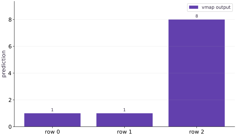
The existing output bars show the lesson's three results, . Their heights check the values; the axis diagram explains how the rows produced them. Compare against an explicit stack of single-row calls, then permute the rows and predict the same permutation of outputs.
Mapped rows and shared weights
Predict: What should happen if you duplicate an input row while keeping the same shared weights?
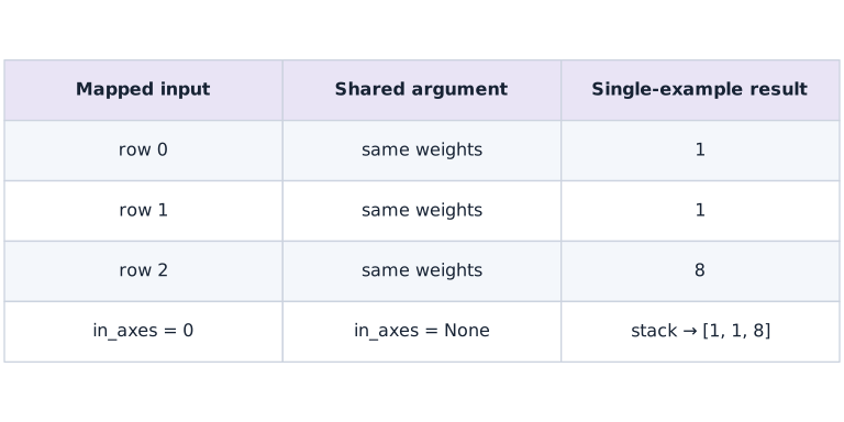
Each row enters the same single-example rule with one shared weight vector. The scalar results are stacked in row order. This is a mathematical mapping, not a hardware-thread allocation. Reordering observations should reorder outputs identically.
Write down the axis contract
There are three independent questions: which dimension represents examples, which inputs should be repeated unchanged, and where should the collected output axis go? and are labels for your reasoning, not named dimensions enforced by JAX.
For the worked example, shared weight is , data is , and predictions are . The first row produces . The second row also produces . The third produces . Calculate those values before reading the batched call.
single: (D,), (D,) → ()
batched: shared (D,), mapped (B,D) → (B,)
Build a reference that is easy to trust
A small Python loop makes the mapping literal: select each data row, call the original function, and stack its results. Keep that reference for tests even if it is not the production implementation. A matrix-vector product is a second independent formulation for this linear model.
Agreement among the loop, vmap, and matrix product checks different ways of describing the same computation. It does not prove that arbitrary future nonlinear models or new axis conventions are correct. Include asymmetric shapes and distinct row values so a transposition or accidentally shared example is easy to detect.
Shared does not mean copied or frozen
None in in_axes tells the transformation that an argument has no mapped axis at this level. Every logical example sees the same parameter value. It is still an argument: you can pass a different weight on the next call. It is not a static compilation argument, and None says nothing about whether a gradient can be computed with respect to it.
Setting both arguments to axis would pair one weight row with one example row. That is useful for an ensemble or a collection of separate models, but it is a different computation from a single shared model. All mapped axes at the same vmap level must have compatible sizes.
Change layout without changing semantics
Some data arrive with examples in columns: shape . Mapping axis selects one column at a time and restores the same single-example shape . in_axes describes that layout. out_axes controls where the new output batch axis is inserted; it does not automatically transpose existing feature dimensions.
For a scalar prediction, output collection gives a vector either way. For a vector-valued feature function, the default produces ; out_axes=1 gives . Keep these distinctions explicit at boundaries between a data loader, model, and loss.
Separate per-example and aggregate gradients
The gradient of a single prediction with respect to its weights is just the input vector. That is a useful first test but not a training loss gradient. A per-example squared error contributes times the input vector. Mapping grad over examples produces an array of shape .
The gradient of the mean loss has shape . For independent example losses and a plain mean reduction, it equals the mean of the per-example gradients. This equivalence is an important check, and it explains why storing all per-example gradients is not necessary for ordinary mean-loss training. Those arrays can be much larger than the aggregate gradient.
Compose transformations around the question
vmap(grad(single_loss)) asks for a gradient per example. grad(mean(vmap(single_loss))) asks for the gradient of a batch objective. Both can be useful, but their output shapes and memory needs differ. Once values match independent references, jit can compile the batched transformed function.
Choose the mathematical quantity first and the transformation order second. Do not copy a composition from a tutorial without checking whether it returns predictions, sensitivities, per-example gradients, or a reduced parameter update.
Vectorization keeps one result per row
Predict before looking: Which observation produces the largest prediction?
Read the figure
Each bar belongs to one input row, and its height is that row’s scalar prediction. Reading left to right gives , , and . The horizontal positions are row labels, not successive training steps.
The same weights are used for every row. The first input gives ; the second gives ; the third gives .
Connect it to the computation
vmap applies the single-example dot product across the batch and keeps one answer per row. Equal heights for the first two bars do not mean those inputs were equal; different inputs can have the same dot product.
There are three outputs because there are three observations. Summing across the whole batch would instead collapse these answers into one scalar. The figure verifies what vectorization computes; the bar heights say nothing about how long it takes.
Open full-size figureDownload data and provenance
The notebook contains the data experiment, plotting code, and recorded figure output. Rerun it to test your changes.
Where to put & run this code: Work in phases/02-transforms/03-batch-a-function-with-vmap/code/main.py (or downloaded exercises/transforms-03.py / exercises/transforms-03.ipynb) and execute from the repository root with python3 phases/02-transforms/03-batch-a-function-with-vmap/code/main.py.
1 Step 1: Set up imports and input tensors
Import the required JAX modules and define the initial inputs for batch a function with vmap.
import jax
import jax.numpy as jnp
Establishing explicit input shapes and dtypes first makes the downstream transformation contract deterministic.
2 Step 2: Apply the core JAX transformation
Write the core computation and transformation step over the initialized inputs.
def predict(weight, x):
    return jnp.dot(weight, x)
weight = jnp.array([2., -1.])
Code building blocks in this step
jnp.array(values, dtype=...)— Constructs an immutable device-backed JAX array from Python/NumPy values.
This stage executes the primary numerical transformation and binds the intermediate outputs.
3 Step 3: Verify shapes and numerical invariants
Check that the resulting arrays satisfy the expected shape, dtype, and numerical tolerances.
batch = jnp.array([[1., 1.], [2., 3.], [4., 0.]])
# Vectorize across the batch dimension with `jax.vmap` (`batched`).
batched = jax.vmap(predict, in_axes=(None, 0))
assert jnp.allclose(batched(weight, batch), jnp.array([1.,1.,8.]))
Code building blocks in this step
jnp.array(values, dtype=...)— Constructs an immutable device-backed JAX array from Python/NumPy values.jnp.allclose(actual, expected, rtol=..., atol=...)— Checks that two arrays match elementwise within floating-point tolerance.jax.vmap(fn, in_axes=..., out_axes=...)— Vectorizes a single-example function across a batch axis without writing a Python loop.
These assertions lock in the exact numerical contract before you run the full experiment and variations.
View the cumulative build in main.py
These blocks append in order to the same file.
import jax
import jax.numpy as jnp

def predict(weight, x):
    return jnp.dot(weight, x)
weight = jnp.array([2., -1.])

batch = jnp.array([[1., 1.], [2., 3.], [4., 0.]])
# Vectorize across the batch dimension with `jax.vmap` (`batched`).
batched = jax.vmap(predict, in_axes=(None, 0))
assert jnp.allclose(batched(weight, batch), jnp.array([1.,1.,8.]))
Run the example
python3 phases/02-transforms/03-batch-a-function-with-vmap/code/main.pyAbout this command
This shortcut uses an activated macOS/Linux course environment in the repository folder. For Windows, use the explicit interpreter command in “Setup help” above. The script includes worked examples and reference solutions.
Inspect the complete assembled example
# Batch a function with vmap: Vectorization lets us describe one example clearly and then...
import jax
import jax.numpy as jnp
def predict(weight, x):
    return jnp.dot(weight, x)
weight = jnp.array([2., -1.])
batch = jnp.array([[1., 1.], [2., 3.], [4., 0.]])
# Vectorize across the batch dimension with `jax.vmap` (`batched`).
batched = jax.vmap(predict, in_axes=(None, 0))
print(batched(weight, batch))
assert jnp.allclose(batched(weight, batch), jnp.array([1.,1.,8.]))
Expected result: [. . .]
Recorded reference execution
Reference output captured from executing the complete lesson script (code/main.py) and its assertions in the course CPU environment.
[1. 1. 8.]
loop / vmap / matmul: [1. 1. 8.] [1. 1. 8.] [1. 1. 8.]
PASS: transforms-03
Download execution record · The notebook includes executed cells and figure outputs. Compare your run with these values; timings depend on the machine.
Verify against a loop and a matrix product
# Experiment — Verify against a loop and a matrix product: The loop makes example selection explicit; the matrix product...
loop_predictions = jnp.stack([predict(weight, row) for row in batch])
vector_predictions = batched(weight, batch)
# Perform matrix / vector contraction (`@`) to compute `matrix_predictions`.
matrix_predictions = batch @ weight
# Check tensor shape invariant: `vector_predictions.shape == (3,)`
assert vector_predictions.shape == (3,)
assert jnp.allclose(vector_predictions, loop_predictions)
assert jnp.allclose(vector_predictions, matrix_predictions)
print("loop / vmap / matmul:", loop_predictions, vector_predictions, matrix_predictions)
Expected: All three formulations produce .
The loop makes example selection explicit; the matrix product checks an independent formulation. Keep both as bounded checks of this linear case.
Move the example axis
# Experiment — Move the example axis: The examples axis and output placement are separate choices.
column_batch = batch.T
# Vectorize across the batch dimension with `jax.vmap` (`column_predict`).
column_predict = jax.vmap(predict, in_axes=(None, 1))
assert jnp.allclose(column_predict(weight, column_batch), vector_predictions)
def feature_pair(row):
    return jnp.array([jnp.sum(row), jnp.sum(row ** 2)])
# Vectorize across the batch dimension with `jax.vmap` (`features_rows`).
features_rows = jax.vmap(feature_pair)(batch)
# Vectorize across the batch dimension with `jax.vmap` (`features_columns`).
features_columns = jax.vmap(feature_pair, out_axes=1)(batch)
# Check tensor shape invariant: `features_rows.shape == (3, 2)`
assert features_rows.shape == (3, 2)
# Check tensor shape invariant: `features_columns.shape == (2, 3)`
assert features_columns.shape == (2, 3)
assert jnp.allclose(features_rows.T, features_columns)
Expected: Column-mapped predictions match the original. Feature layouts are and .
The examples axis and output placement are separate choices. Use values as well as shapes to verify a layout change.
Make it yours
Where to put your code: Append your solution at the bottom of phases/02-transforms/03-batch-a-function-with-vmap/code/main.py (or inside the Make it yours cell of exercises/transforms-03.ipynb) and run python3 phases/02-transforms/03-batch-a-function-with-vmap/code/main.py to verify your prediction before opening the reference solution.
Foundation · Compute each prediction gradient with respect to the shared weight. Predict the shape and the derivative of the dot product, then verify against the input batch.
Show a writing guide and starter scaffold
How to write this exercise code: step-by-step recipe & starter scaffold
1. Key functions & syntax to use:
jnp.allclose(actual, expected, rtol=..., atol=...)— Checks that two arrays match elementwise within floating-point tolerance.jax.grad(loss_fn)(params, ...)— Transforms a scalar-output function into a function returning the gradient PyTree with the same structure asparams.jax.vmap(fn, in_axes=..., out_axes=...)— Vectorizes a single-example function across a batch axis without writing a Python loop.
2. Step-by-step implementation plan:
- Differentiate the objective to obtain
per_example_gradientvia automatic differentiation. - Check tensor shape invariant:
per_example_gradient.shape == (3, 2)
# Exercise solution: Foundation · Compute each prediction gradient with respect to the...
# Differentiate the objective to obtain `per_example_gradient` via automatic differentiation.
per_example_gradient = jax.vmap(...)  # TODO: compute per_example_gradient
# Check tensor shape invariant: `per_example_gradient.shape == (3, 2)`
assert per_example_gradient.shape  # TODO: complete assertion check
assert jnp.allclose(per_example_gradient, batch)  # TODO: complete assertion check
Reveal the reference solution
# Exercise solution: Foundation · Compute each prediction gradient with respect to the...
# Differentiate the objective to obtain `per_example_gradient` via automatic differentiation.
per_example_gradient = jax.vmap(jax.grad(predict), in_axes=(None, 0))(weight, batch)
# Check tensor shape invariant: `per_example_gradient.shape == (3, 2)`
assert per_example_gradient.shape == (3, 2)
assert jnp.allclose(per_example_gradient, batch)
Turn sensitivities into training gradients
Practice
Use targets . Define a scalar squared-error function for one example. Compute all per-example parameter gradients and derive the first row independently.
Show a writing guide and starter scaffold
How to write this practice solution: step-by-step recipe & starter scaffold
1. Key functions & syntax to use:
jnp.array(values, dtype=...)— Constructs an immutable device-backed JAX array from Python/NumPy values.jnp.allclose(actual, expected, rtol=..., atol=...)— Checks that two arrays match elementwise within floating-point tolerance.jax.grad(loss_fn)(params, ...)— Transforms a scalar-output function into a function returning the gradient PyTree with the same structure asparams.jax.vmap(fn, in_axes=..., out_axes=...)— Vectorizes a single-example function across a batch axis without writing a Python loop.
2. Step-by-step implementation plan:
- Differentiate the objective to obtain
individual_gradsvia automatic differentiation. - Check tensor shape invariant:
individual_grads.shape == (3, 2)
# Turn sensitivities into training gradients (Practice): The first residual is 1, so the first loss gradient is [2, 2].
targets = jnp.array(...)  # TODO: compute targets
def single_loss(parameters, row, target):
    return ...  # TODO: return computed result
# Differentiate the objective to obtain `individual_grads` via automatic differentiation.
individual_grads = jax.vmap(...)  # TODO: compute individual_grads
manual_grads = ...  # TODO: compute manual_grads
# Check tensor shape invariant: `individual_grads.shape == (3, 2)`
assert individual_grads.shape  # TODO: complete assertion check
assert jnp.allclose(individual_grads, manual_grads)  # TODO: complete assertion check
assert jnp.allclose(individual_grads[0], jnp.array([2., 2.]))  # TODO: complete assertion check
Show a hint
The per-example squared-loss gradient is : twice the residual times the input. A prediction gradient by itself is not a loss gradient.
Reveal reference solution and reasoning
# Turn sensitivities into training gradients (Practice): The first residual is 1, so the first loss gradient is [2, 2].
targets = jnp.array([0., 2., 7.])
def single_loss(parameters, row, target):
    return (predict(parameters, row) - target) ** 2
# Differentiate the objective to obtain `individual_grads` via automatic differentiation.
individual_grads = jax.vmap(jax.grad(single_loss), in_axes=(None, 0, 0))(weight, batch, targets)
manual_grads = 2. * (batch @ weight - targets)[:, None] * batch
# Check tensor shape invariant: `individual_grads.shape == (3, 2)`
assert individual_grads.shape == (3, 2)
assert jnp.allclose(individual_grads, manual_grads)
assert jnp.allclose(individual_grads[0], jnp.array([2., 2.]))
The first residual is , so the first loss gradient is . The batch axis records three separate contributions.
Prove the mean-gradient identity with an experiment
Challenge
Define the mean loss from the mapped single loss. Compare its parameter gradient with the mean of individual_grads. Repeat after changing targets and explain why a sum changes the relationship.
Show a writing guide and starter scaffold
How to write this practice solution: step-by-step recipe & starter scaffold
1. Key functions & syntax to use:
x.sum(axis=...) / x.mean(axis=..., keepdims=...)— Reduces values along the namedaxis(the axis you name is collapsed unlesskeepdims=True).jnp.allclose(actual, expected, rtol=..., atol=...)— Checks that two arrays match elementwise within floating-point tolerance.jax.grad(loss_fn)(params, ...)— Transforms a scalar-output function into a function returning the gradient PyTree with the same structure asparams.jax.vmap(fn, in_axes=..., out_axes=...)— Vectorizes a single-example function across a batch axis without writing a Python loop.
2. Step-by-step implementation plan:
- Differentiate the objective to obtain
eachvia automatic differentiation. - Differentiate the objective to obtain
aggregatevia automatic differentiation. - Check tensor shape invariant:
aggregate.shape == weight.shape
# Prove the mean-gradient identity with an experiment (Challenge): The aggregate has parameter shape, while per-example...
def batch_mean_loss(parameters, rows, labels):
    return jnp.mean(jax.vmap(single_loss, in_axes = ...  # TODO: compute return jnp.mean(jax.vmap(single_loss, in_axes
for labels in (targets, targets + 0.5):
    # Differentiate the objective to obtain `each` via automatic differentiation.
    each = jax.vmap(...)  # TODO: compute each
    # Differentiate the objective to obtain `aggregate` via automatic differentiation.
    aggregate = jax.grad(...)  # TODO: compute aggregate
    # Check tensor shape invariant: `aggregate.shape == weight.shape`
    assert aggregate.shape  # TODO: complete assertion check
    assert jnp.allclose(aggregate, jnp.mean(each, axis=0))  # TODO: complete assertion check
Show a hint
Differentiation is linear over these independent sums. Ensure your function actually averages over the example axis.
Reveal reference solution and reasoning
# Prove the mean-gradient identity with an experiment (Challenge): The aggregate has parameter shape, while per-example...
def batch_mean_loss(parameters, rows, labels):
    return jnp.mean(jax.vmap(single_loss, in_axes=(None, 0, 0))(parameters, rows, labels))
for labels in (targets, targets + 0.5):
    # Differentiate the objective to obtain `each` via automatic differentiation.
    each = jax.vmap(jax.grad(single_loss), in_axes=(None, 0, 0))(weight, batch, labels)
    # Differentiate the objective to obtain `aggregate` via automatic differentiation.
    aggregate = jax.grad(batch_mean_loss)(weight, batch, labels)
    # Check tensor shape invariant: `aggregate.shape == weight.shape`
    assert aggregate.shape == weight.shape
    assert jnp.allclose(aggregate, jnp.mean(each, axis=0))
The aggregate has parameter shape, while per-example gradients add an examples axis. This identity relies on the stated independent-example loss and mean reduction, not on every model that has a batch dimension.
Diagnose the result
If mapped axes have inconsistent sizes, inspect every mapped input before changing the model. If dot-product shapes fail, check whether you selected a row or a column. If gradients have an unexpected examples axis, distinguish a mapped gradient from the gradient of a reduced loss. If an implementation seems faster, first establish value equivalence and use the synchronized benchmark procedure from the next lesson.
Carry forward
- Reason about one example before describing the batch axis.
in_axes=Noneshares an input at that map level; it does not make it static or nondifferentiable.- A loop reference and asymmetric data expose many axis mistakes.
- Per-example gradients and aggregate gradients answer different questions.
Keep your evidence
Keep the shape contract, loop/vmap/matrix equivalence, row/column layout checks, per-example gradient array, and mean-gradient identity under two target sets. Explain what each gradient shape means.
Save your modified code, its output, and an explanation of your prediction. Checkpoint answers and exercise evidence are tracked separately.
Saved in this browser. Export or back up your portfolio anytime in My learning.
Verified on local CPU. Stage to a Cloud TPU VM via Cloud TPU setup to record accelerator execution receipts (TODO: add automated Cloud TPU CI execution receipts).