 JAX Pathways
Phase 02 / JAX transformations
Compile a function with jit
Revision v0.7.0 · Updated since your last visit. Review the changes; your progress is saved.
Lesson · about 55 minutes · CPU practice
Validate compiled loss/gradient values and produce a correctly synchronized latency report.
Phase study guide: preparation, milestones and project evidence
Before you start
Before this: Batch a function with vmap
Hardware: CPU
Setup help: Python, notebook, or Cloud TPU VM
Use the tested CPU packages (the recorded environment uses Python 3.14.3). Other Python versions and accelerator environments require separate checks. The optional Cloud TPU specialization explains the target-specific execution boundaries. Logical CPU devices practice partitioning; they do not simulate TPU performance.
Download the repository ZIP or use your existing checkout. Extract it and open a terminal in the folder containing requirements-cpu.txt. The beginner ZIP is separate; these lessons use the full repository folder.
python3 -m venv .venv
source .venv/bin/activate
python -m pip install -r requirements-cpu.txtpy -3 -m venv .venv
.\.venv\Scripts\python.exe -m pip install -r requirements-cpu.txtAfter activation, run the complete worked example from that same folder:
python phases/02-transforms/04-compile-a-function-with-jit/code/main.py.\.venv\Scripts\python.exe phases/02-transforms/04-compile-a-function-with-jit/code/main.pyFor an incremental build, create main.py in your own practice folder, append each build block in order, and run python main.py with this environment active. Keep that file separate from the downloaded reference solution.
Download this lesson’s notebook. Open it with a Python kernel using the course environment. Run cells from the top after restarting the kernel; experiments depend on earlier definitions.
For local Jupyter, first install the course requirements using the Local Python steps, then use your environment’s Python to start Jupyter:
python -m pip install jupyterlab
python -m jupyter lab.\.venv\Scripts\python.exe -m pip install jupyterlab
.\.venv\Scripts\python.exe -m jupyter labSelect the downloaded transforms-04.ipynb file in JupyterLab. The notebook contains reference solutions; make your prediction and attempt each practice task before opening them. Restart the kernel before changing logical device setup.
The worked reference for this lesson is CPU-validated. Some references explicitly configure logical CPU devices; setting JAX_PLATFORMS does not adapt them to a TPU. Follow the execution matrix and reviewed multi-host example before attempting a target run.
For accelerator preparation, study TPU setup, observed runtime receipts, checkpointed jobs and precision and retained traces. These target paths remain unqualified on physical TPU hardware until an actual receipt is recorded. Cloud provisioning is optional for CPU learning.
Check: Loss ≈ . Timings depend on the device, process, and workload; no speed threshold is required.
Revisit the guided CPU setup · Open 19: TPU Setup. Package instructions are CPU instructions; Windows and accelerator environments need their own validation.
What you will be able to do
- Explain tracing, compilation, dispatch, and synchronization as separate work.
- Validate a compiled numerical function against its eager and analytic results.
- Measure first-call latency and repeated-call latency with explicit completion.
- Compile a value-and-gradient computation without claiming a universal speedup.
The problem
Your calculation is correct, and now you want to run it many times. What does compilation actually change? We’ll compare the original function with its jitted version, separate the first call from later calls, and wait for the result before stopping the timer. A small CPU example is enough to learn a fair comparison; a speedup is not guaranteed.
The idea
Compilation prepares a program that can be reused for compatible calls. The first call can include tracing and compilation as well as execution; later compatible calls can reuse that work. Numerical equality and performance are separate checks.
Separate changing data from preparing a program
Suppose you call a compiled function on a float32 vector, then call it on different values with the same shape and dtype. Those new values can flow through the prepared computation. If the next call changes a relevant shape or static choice, JAX may need a different specialization.
Think of the first-call path as preparation followed by execution. A warm-call timing should describe the repeated workload after preparation, and it must wait for device work to finish. Timing only dispatch can make a slow computation look fast.
First compare compiled and ordinary outputs on several inputs. Then, if speed is your question, state the input size, device, warmup and synchronization boundary. Three equal bars demonstrate agreement; they do not demonstrate acceleration.
Separate the work hidden in one call
The first call can involve tracing, lowering, compilation, dispatch, and execution. Calling the same compiled function on compatible inputs can avoid much of the setup, but still involves a Python invocation, dispatch, and execution. A persistent cache or earlier compilation can also affect what first means.
Define the scope: first call to this callable in this process with these input shapes/dtypes. Do not label it cold-machine startup, pure compilation time, or kernel execution time unless your experiment actually isolates those quantities.
first relevant call → trace / compile / dispatch / execute
compatible repeated call → reuse / dispatch / execute
Check values before timing
Our input matrix has shape , weights have shape , and targets have shape . Predictions are . Residuals are . Squaring and averaging yields . Compute this independently so that two implementations agreeing on an unintended broadcast is not mistaken for correctness.
Compilation should preserve the intended numerical calculation within suitable tolerance. Floating-point transformations and reduction ordering can change last bits; exact equality is often too strong. Choose tolerance using dtype and scale, and do not suppress large discrepancies with a very loose allclose check.
Wait for the quantity you are timing
JAX can return an array object while device computation is still pending. Timing only the Python call can therefore measure dispatch rather than completed work. block_until_ready waits for the array result without needing to print it or convert it to NumPy.
A function returning a tuple or a parameter tree needs a completion strategy for all relevant leaves. A scalar loss is convenient for this introductory experiment because waiting on it marks that result complete. Keep data creation and transfers outside the interval when measuring a prepared numerical invocation; include them deliberately when measuring end-to-end latency.
Use repetitions and report a distribution
One repeated call is easy to distort with scheduling noise. Warm the exact callable and input signature, collect multiple completion-synchronized durations, and report a median plus range and repeat count. Use the same prepared arrays and comparable waiting behavior for eager and compiled calls.
This measures invocation latency under the stated conditions, including Python overhead. It is not a throughput measurement for queued training steps, and it does not isolate accelerator kernels. A median for a small toy workload cannot justify a performance claim about your future model or a different device.
Compile the computation you intend to repeat
For training, loss and parameter gradients are often consumed together. jit(value_and_grad(loss)) expresses a compiled transformed computation that returns both. Check the value against the loss and the gradient against an independent formula before using it as part of an update.
Avoid creating a fresh jitted lambda inside every iteration. Reusing a stable transformed callable gives compilation reuse a chance. A useful compilation boundary often surrounds a complete step rather than every scalar operation, but the correct boundary depends on the workload, state, and integration constraints. We will make state explicit before building that larger step.
Decide when compilation is worth its setup
A long compilation can be worthwhile if a computation runs many times. A one-off small calculation might never recover its setup cost. You need both setup latency and steady-state measurements to reason about break-even behavior.
This lesson does not measure TPU execution, multi-device scaling, or a model training speedup. Its artifact is a reproducible correctness/timing report that records the backend, shapes, dtype, synchronization policy, warmup, repeat count, and observed durations.
Compilation preserves the result
Predict before looking: Should compilation change the loss value?
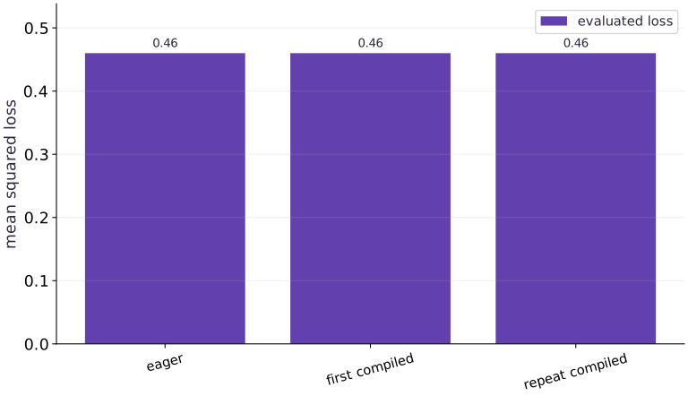
Read the figure
The three categories are eager execution, the first compiled call, and a repeated compiled call. The vertical axis is mean squared loss. Each bar reaches approximately , so all three execution paths return the same numerical result for this input.
These are separate bars with equal heights. The first compiled call has not disappeared, and its bar is not a measurement of compilation time.
Connect it to the computation
Compilation changes how the computation runs while preserving its intended result. The agreement here is the correctness check to make before asking whether compilation improved performance. Small floating-point differences should be assessed with the example’s numerical tolerance.
To measure speed, you need a time axis, synchronization, warm-up, and repeated measurements. None of those can be inferred from these loss bars. A useful next check is to change the input values and confirm that eager and compiled results still agree.
Open full-size figureDownload data and provenance
The notebook contains the data experiment, plotting code, and recorded figure output. Rerun it to test your changes.
Where to put & run this code: Work in phases/02-transforms/04-compile-a-function-with-jit/code/main.py (or downloaded exercises/transforms-04.py / exercises/transforms-04.ipynb) and execute from the repository root with python3 phases/02-transforms/04-compile-a-function-with-jit/code/main.py.
1 Step 1: Set up imports and input tensors
Import the required JAX modules and define the initial inputs for compile a function with jit.
import time
import jax
import jax.numpy as jnp
def loss(w, x, y):
    return jnp.mean((x @ w - y) ** 2)
# Construct and reshape `x` into the target tensor dimensions.
x = jnp.arange(12, dtype=jnp.float32).reshape(4, 3) / 10.
Code building blocks in this step
jnp.arange(n, dtype=...)— Creates a 1-D JAX array of evenly spaced values[0, 1, ..., n-1]on the target device.array.reshape(new_shape)— Reorganizes tensor axes without changing the total element count (array.size).x.sum(axis=...) / x.mean(axis=..., keepdims=...)— Reduces values along the namedaxis(the axis you name is collapsed unlesskeepdims=True).
Establishing explicit input shapes and dtypes first makes the downstream transformation contract deterministic.
2 Step 2: Apply the core JAX transformation
Write the core computation and transformation step over the initialized inputs.
w = jnp.array([1., 2., -1.])
y = jnp.ones(4)
# Wrap with `jax.jit` (`compiled`) so XLA traces and compiles the function.
compiled = jax.jit(loss)
t0 = time.perf_counter()
# Synchronize host execution until asynchronous device computation completes.
first = compiled(w, x, y).block_until_ready()
Code building blocks in this step
jnp.array(values, dtype=...)— Constructs an immutable device-backed JAX array from Python/NumPy values.jnp.zeros / jnp.ones(shape, dtype=...)— Allocates a tensor of the givenshapeinitialized with constants.jax.jit(fn) / @jax.jit— Tracesfnwith abstract shapes and compiles a fused XLA executable cached by input shape and dtype.jax.block_until_ready(output)— Synchronizes with the accelerator/CPU device so asynchronous dispatch finishes before wall-clock timing.
This stage executes the primary numerical transformation and binds the intermediate outputs.
3 Step 3: Verify shapes and numerical invariants
Check that the resulting arrays satisfy the expected shape, dtype, and numerical tolerances.
first_seconds = time.perf_counter() - t0
t0 = time.perf_counter()
# Synchronize host execution until asynchronous device computation completes.
second = compiled(w, x, y).block_until_ready()
repeat_seconds = time.perf_counter() - t0
assert jnp.allclose(first, loss(w, x, y))
assert jnp.allclose(second, first)
Code building blocks in this step
jnp.allclose(actual, expected, rtol=..., atol=...)— Checks that two arrays match elementwise within floating-point tolerance.jax.block_until_ready(output)— Synchronizes with the accelerator/CPU device so asynchronous dispatch finishes before wall-clock timing.
These assertions lock in the exact numerical contract before you run the full experiment and variations.
View the cumulative build in main.py
These blocks append in order to the same file.
import time
import jax
import jax.numpy as jnp
def loss(w, x, y):
    return jnp.mean((x @ w - y) ** 2)
# Construct and reshape `x` into the target tensor dimensions.
x = jnp.arange(12, dtype=jnp.float32).reshape(4, 3) / 10.

w = jnp.array([1., 2., -1.])
y = jnp.ones(4)
# Wrap with `jax.jit` (`compiled`) so XLA traces and compiles the function.
compiled = jax.jit(loss)
t0 = time.perf_counter()
# Synchronize host execution until asynchronous device computation completes.
first = compiled(w, x, y).block_until_ready()

first_seconds = time.perf_counter() - t0
t0 = time.perf_counter()
# Synchronize host execution until asynchronous device computation completes.
second = compiled(w, x, y).block_until_ready()
repeat_seconds = time.perf_counter() - t0
assert jnp.allclose(first, loss(w, x, y))
assert jnp.allclose(second, first)
Run the example
python3 phases/02-transforms/04-compile-a-function-with-jit/code/main.pyAbout this command
This shortcut uses an activated macOS/Linux course environment in the repository folder. For Windows, use the explicit interpreter command in “Setup help” above. The script includes worked examples and reference solutions.
Inspect the complete assembled example
# Compile a function with jit: Compilation prepares a program that can be reused for compatible...
import time
import jax
import jax.numpy as jnp
def loss(w, x, y):
    return jnp.mean((x @ w - y) ** 2)
# Construct and reshape `x` into the target tensor dimensions.
x = jnp.arange(12, dtype=jnp.float32).reshape(4, 3) / 10.
w = jnp.array([1., 2., -1.])
y = jnp.ones(4)
# Wrap with `jax.jit` (`compiled`) so XLA traces and compiles the function.
compiled = jax.jit(loss)
t0 = time.perf_counter()
# Synchronize host execution until asynchronous device computation completes.
first = compiled(w, x, y).block_until_ready()
first_seconds = time.perf_counter() - t0
t0 = time.perf_counter()
# Synchronize host execution until asynchronous device computation completes.
second = compiled(w, x, y).block_until_ready()
repeat_seconds = time.perf_counter() - t0
print("Loss:", float(second))
print("First/repeat seconds:", first_seconds, repeat_seconds)
assert jnp.allclose(first, loss(w, x, y))
assert jnp.allclose(second, first)
Expected result: Loss ≈ . Timings depend on the device, process, and workload; no speed threshold is required.
Recorded reference execution
Reference output captured from executing the complete lesson script (code/main.py) and its assertions in the course CPU environment.
Loss: 0.46000000834465027
First/repeat seconds: 0.013900000136345625 1.920759677886963e-05
eager median / min / max seconds: 2.6375288143754005e-05 2.3334287106990814e-05 7.895799353718758e-05
compiled median / min / max seconds: 4.312489181756973e-06 3.874767571687698e-06 5.416106432676315e-06
backend / shapes / dtype: cpu (4, 3) (3,) (4,) float32
compiled value-and-grad median seconds: 6.770249456167221e-06
PASS: transforms-04
Download execution record · The notebook includes executed cells and figure outputs. Compare your run with these values; timings depend on the machine.
Derive predictions and gradients outside the transform
# Experiment — Derive predictions and gradients outside the transform: The analytic value check detects mistakes that...
expected_predictions = jnp.array([0., 0.6, 1.2, 1.8])
assert jnp.allclose(x @ w, expected_predictions, atol=1e-6)
assert jnp.allclose(compiled(w, x, y), 0.46, atol=1e-6)
# Perform matrix / vector contraction (`@`) to compute `manual_gradient`.
manual_gradient = (2. / len(y)) * x.T @ (x @ w - y)
# Differentiate the objective to obtain `compiled_value_gradient` via automatic differentiation.
compiled_value_gradient = jax.jit(jax.value_and_grad(loss))
checked_value, checked_gradient = compiled_value_gradient(w, x, y)
assert jnp.allclose(checked_gradient, manual_gradient, rtol=1e-5, atol=1e-6)
Expected: The loss is ; the gradient matches the independent matrix expression.
The analytic value check detects mistakes that eager-versus-compiled equality alone would miss.
Collect a synchronized latency sample
# Experiment — Collect a synchronized latency sample: The report includes Python invocation and completed numerical...
import statistics
def completed_samples(function, repeats=20):
    # Synchronize host execution until asynchronous device computation completes.
    function(w, x, y).block_until_ready()
    durations = []
    for _ in range(repeats):
        start = time.perf_counter()
        # Synchronize host execution until asynchronous device computation completes.
        function(w, x, y).block_until_ready()
        durations.append(time.perf_counter() - start)
    return durations
for name, function in (("eager", loss), ("compiled", compiled)):
    samples = completed_samples(function)
    print(name, "median / min / max seconds:", statistics.median(samples), min(samples), max(samples))
print("backend / shapes / dtype:", jax.default_backend(), x.shape, w.shape, y.shape, x.dtype)
Expected: Twenty completed calls are measured after a warmup for each callable. Durations vary; no speed threshold is asserted.
The report includes Python invocation and completed numerical work on already prepared data. It is a bounded latency observation, not a universal accelerator benchmark.
Make it yours
Where to put your code: Append your solution at the bottom of phases/02-transforms/04-compile-a-function-with-jit/code/main.py (or inside the Make it yours cell of exercises/transforms-04.ipynb) and run python3 phases/02-transforms/04-compile-a-function-with-jit/code/main.py to verify your prediction before opening the reference solution.
Foundation · Compile value_and_grad(loss), check the loss and gradient against both the eager transform and the manual matrix formula, and explain how you would synchronize a benchmark of its two outputs.
Show a writing guide and starter scaffold
How to write this exercise code: step-by-step recipe & starter scaffold
1. Key functions & syntax to use:
jnp.allclose(actual, expected, rtol=..., atol=...)— Checks that two arrays match elementwise within floating-point tolerance.jax.value_and_grad(loss_fn)(params, ...)— Evaluates both the scalar loss and its gradient PyTree(loss_val, grads)in a single forward+backward pass.jax.jit(fn) / @jax.jit— Tracesfnwith abstract shapes and compiles a fused XLA executable cached by input shape and dtype.
2. Step-by-step implementation plan:
- Differentiate the objective to obtain
compiled_stepvia automatic differentiation. - Differentiate the objective to obtain
(expected_v, expected_g)via automatic differentiation.
# Exercise solution: Foundation · Compile value_and_grad(loss), check the loss and gradient...
# Differentiate the objective to obtain `compiled_step` via automatic differentiation.
compiled_step = jax.jit(...)  # TODO: compute compiled_step
v, g = compiled_step(...)  # TODO: compute v, g
# Differentiate the objective to obtain `(expected_v, expected_g)` via automatic differentiation.
expected_v, expected_g = jax.value_and_grad(...)  # TODO: compute expected_v, expected_g
assert jnp.allclose(v, expected_v)  # TODO: complete assertion check
assert jnp.allclose(g, expected_g)  # TODO: complete assertion check
Reveal the reference solution
# Exercise solution: Foundation · Compile value_and_grad(loss), check the loss and gradient...
# Differentiate the objective to obtain `compiled_step` via automatic differentiation.
compiled_step = jax.jit(jax.value_and_grad(loss))
v, g = compiled_step(w, x, y)
# Differentiate the objective to obtain `(expected_v, expected_g)` via automatic differentiation.
expected_v, expected_g = jax.value_and_grad(loss)(w, x, y)
assert jnp.allclose(v, expected_v)
assert jnp.allclose(g, expected_g)
Check that a new value remains runtime data
Practice
Keep shapes and dtypes fixed, change , and compare the compiled loss against an independently computed residual mean. Explain why a different numerical answer does not itself imply a new compilation.
Show a writing guide and starter scaffold
How to write this practice solution: step-by-step recipe & starter scaffold
1. Key functions & syntax to use:
x.sum(axis=...) / x.mean(axis=..., keepdims=...)— Reduces values along the namedaxis(the axis you name is collapsed unlesskeepdims=True).jnp.allclose(actual, expected, rtol=..., atol=...)— Checks that two arrays match elementwise within floating-point tolerance.
2. Step-by-step implementation plan:
- Aggregate array values to compute
expected.
# Check that a new value remains runtime data (Practice): The same computation accepts different runtime values.
for new_w in (w, w + 0.25):
    # Aggregate array values to compute `expected`.
    expected = jnp.mean(...)  # TODO: compute expected
    observed = compiled(...)  # TODO: compute observed
    assert jnp.allclose(observed, expected, rtol=1e-5, atol=1e-6)  # TODO: complete assertion check
Show a hint
Compilation specializes to relevant properties, not each ordinary array element value.
Reveal reference solution and reasoning
# Check that a new value remains runtime data (Practice): The same computation accepts different runtime values.
for new_w in (w, w + 0.25):
    # Aggregate array values to compute `expected`.
    expected = jnp.mean((x @ new_w - y) ** 2)
    observed = compiled(new_w, x, y)
    assert jnp.allclose(observed, expected, rtol=1e-5, atol=1e-6)
The same computation accepts different runtime values. The next lesson inspects tracing explicitly rather than inferring it from timing noise.
Build a report whose timing claim can be checked
Challenge
Benchmark the compiled value-and-gradient function for calls after warmup, waiting on every output leaf. Include backend, input shapes, dtype, and median. State what your measurement excludes.
Show a writing guide and starter scaffold
How to write this practice solution: step-by-step recipe & starter scaffold
1. Key functions & syntax to use:
jax.tree.map(lambda p, g: ..., params, grads)— Applies a function leaf-by-leaf across matching PyTrees (such as updating every parameter tensor with its gradient).jax.block_until_ready(output)— Synchronizes with the accelerator/CPU device so asynchronous dispatch finishes before wall-clock timing.
2. Step-by-step implementation plan:
- Set up the changed input or configuration parameters requested in the prompt.
- Run the target function or transformation and assert that the output matches your prediction.
# Build a report whose timing claim can be checked (Challenge): The measurement excludes input construction and first...
def wait_for_outputs(outputs):
    return ...  # TODO: return computed result
wait_for_outputs(compiled_value_gradient(w, x, y))
gradient_times = ...  # TODO: compute gradient_times
for _ in range(20):
    started = time.perf_counter(...)  # TODO: compute started
    wait_for_outputs(compiled_value_gradient(w, x, y))
    gradient_times.append(time.perf_counter() - started)
print("compiled value-and-grad median seconds:", statistics.median(gradient_times))
assert len(gradient_times)  # TODO: complete assertion check
Show a hint
Use jax.tree.map to block on every returned array, then stop the timer.
Reveal reference solution and reasoning
# Build a report whose timing claim can be checked (Challenge): The measurement excludes input construction and first...
def wait_for_outputs(outputs):
    return jax.tree.map(lambda array: array.block_until_ready(), outputs)
wait_for_outputs(compiled_value_gradient(w, x, y))
gradient_times = []
for _ in range(20):
    started = time.perf_counter()
    wait_for_outputs(compiled_value_gradient(w, x, y))
    gradient_times.append(time.perf_counter() - started)
print("compiled value-and-grad median seconds:", statistics.median(gradient_times))
assert len(gradient_times) == 20
The measurement excludes input construction and first compilation, and includes repeated invocation and completion. It cannot be compared with another report without matching those boundaries.
Diagnose the result
A suspiciously tiny time may measure dispatch only; inspect synchronization. A slow first call followed by faster calls may reflect setup, but timing alone does not identify which setup stage. Inconsistent eager/compiled results call for shape, dtype, and tolerance checks before performance tuning. Repeatedly slow setup can come from recreating transformed functions or changing specialization inputs; the next lesson tests those hypotheses directly.
Carry forward
- Compilation setup and repeated invocation are different measurements.
- Correctness needs independent numerical checks before performance interpretation.
- Asynchronous execution requires completion synchronization.
- A useful report records workload, backend, dtype, warmup, repetitions, and timing boundaries.
Keep your evidence
Keep the independent loss/gradient calculation, backend/shapes/dtype, first-call interval, warmup/repeat policy, median/range samples, and synchronization of every output leaf. State what the benchmark excludes.
Save your modified code, its output, and an explanation of your prediction. Checkpoint answers and exercise evidence are tracked separately.
Saved in this browser. Export or back up your portfolio anytime in My learning.
Verified on local CPU. Stage to a Cloud TPU VM via Cloud TPU setup to record accelerator execution receipts (TODO: add automated Cloud TPU CI execution receipts).