Systems Specialization · CPU ReferenceCPU reference; target qualification separateLesson 7 of 8 in Phase 15

Phase 15 / Deployment, interoperability & edge AI

Inference capacity, batching, and autoscaling

Revision v0.7.0 · 2026-10-20

Lesson · about 130 minutes · CPU practice

Measure completed inference after warming each batch shape Report batch latency and example throughput with correct units

Phase study guide: preparation, milestones and project evidence

Before you start

Before this: Containerize a model service and verify its boundary
Hardware: CPU

Download notebook

Other downloads

Python worked examples Lesson text

Setup help: Python, notebook, or Cloud TPU VM

Use the tested CPU packages (the recorded environment uses Python 3.14.3). Other Python versions and accelerator environments require separate checks. The optional Cloud TPU specialization explains the target-specific execution boundaries. Logical CPU devices practice partitioning; they do not simulate TPU performance.

Download the repository ZIP or use your existing checkout. Extract it and open a terminal in the folder containing requirements-cpu.txt. The beginner ZIP is separate; these lessons use the full repository folder.

macOS / Linux terminal · repository folder

python3 -m venv .venv
source .venv/bin/activate
python -m pip install -r requirements-cpu.txt

PowerShell · repository folder

py -3 -m venv .venv
.\.venv\Scripts\python.exe -m pip install -r requirements-cpu.txt

After activation, run the complete worked example from that same folder:

macOS / Linux terminal · activated environment

python phases/15-deployment/04-inference-capacity-batching-and-autoscaling/code/main.py

PowerShell command · repository folder

.\.venv\Scripts\python.exe phases/15-deployment/04-inference-capacity-batching-and-autoscaling/code/main.py

For an incremental build, create main.py in your own practice folder, append each build block in order, and run python main.py with this environment active. Keep that file separate from the downloaded reference solution.

Download this lesson’s notebook. Open it with a Python kernel using the course environment. Run cells from the top after restarting the kernel; experiments depend on earlier definitions.

For local Jupyter, first install the course requirements using the Local Python steps, then use your environment’s Python to start Jupyter:

macOS / Linux terminal · activated course environment

python -m pip install jupyterlab
python -m jupyter lab

PowerShell command · repository folder

.\.venv\Scripts\python.exe -m pip install jupyterlab
.\.venv\Scripts\python.exe -m jupyter lab

Select the downloaded deployment-04.ipynb file in JupyterLab. The notebook contains reference solutions; make your prediction and attempt each practice task before opening them. Restart the kernel before changing logical device setup.

Check: The program prints first-call, warm p50/p95 and examples-per-second measurements for each batch size. Absolute timings are host-dependent. The independent queue example yields response times of 2, 3 and 2 milliseconds.

Revisit the guided CPU setup · Open 19: TPU Setup. Package instructions are CPU instructions; Windows and accelerator environments need their own validation.

Phase 15.07 Stage 1 of 5 · Understand

1 Understand 2 Build & Run 3 Experiment 4 Exercise & Check 5 Evidence

What you will be able to do

Measure completed inference after warming each batch shape
Report batch latency and example throughput with correct units
Implement and independently check a serial queue timeline
Distinguish utilization, batch-collection delay and hypothetical replica planning from measured service evidence

The problem

A model call looks fast in isolation, yet users may wait when requests arrive together. We will measure actual completed inference at several batch sizes, then use those observations in a clearly labeled queue simulation. The aim is to connect milliseconds per batch, examples per second and response latency without confusing a local benchmark with a deployed service.

The idea

Inference capacity depends on arrivals, queueing, batching, service time and response work. A fast model call is one component. Define the request boundary before estimating throughput or deciding when to add capacity.

A request spends time before and after computation

A request may wait for a batch, wait behind existing work, execute and then be encoded for response. Larger batches can improve work per call while increasing the first waiting request's latency. These objectives can conflict.

Draw arrival, enqueue, dispatch and completion on one timeline. Then measure or model each interval with its source stated. Tail latency depends on the arrival pattern and concurrency, not just the mean of isolated calls.

This lesson combines measured CPU batch computation with a separately simulated queue. Keep those panels distinct. A queue simulation explores stated assumptions; it is not an observed autoscaling system or a production traffic measurement.

Choose the clock boundary first

JAX dispatch may return before numerical work has completed. The timer calls block_until_ready inside the measured interval. Inputs and weights are already resident; preprocessing, device placement, request decoding and response encoding are excluded. The first call for each shape can include compilation and is recorded separately from $40$ warm calls. A p95 from $40$ samples is a small descriptive statistic, not a reliable production tail estimate. Timings change across hosts and repeated runs; correctness checks must not assert a fixed speedup.

Keep request units and example units separate

Let a batch of $B$ examples take $t_B$ milliseconds. A serial worker completing full batches has a compute-throughput proxy $1000B/t_B$ examples per second. The batch still takes $t_B$ milliseconds; dividing by $B$ describes amortized cost per example, not the response time experienced by one example in that batch. Partial batches, memory pressure, shape recompilation and preprocessing can change both numbers.

q_B=\frac{1000B}{t_B}\quad\text{examples/second}

Trace a queue before using a rate formula

For one first-come-first-served worker, a request starts at the later of its arrival and the previous finish. With arrivals at $0,1,4$ milliseconds and service duration $2$ milliseconds, starts are $0,2,4$ , finishes are $2,4,6$ , and response times are $2,3,2$ . The second request waits one millisecond because the worker is busy. This independent hand timeline checks our simulation before we feed it measured service durations.

s_i=\max(a_i,f_{i-1}),\qquad f_i=s_i+t,\qquad r_i=f_i-a_i

A utilization estimate is not a latency guarantee

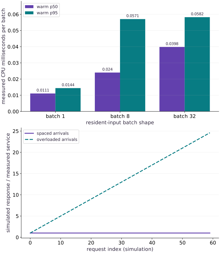
If arrival rate is $\lambda$ requests per second and each request consumes $t$ milliseconds on one serial worker, the utilization proxy is $\rho=\lambda t/1000$ . Sustained offered work above capacity makes backlog grow in this unlimited-queue model. Even below capacity, bursts and service-time variation can cause long waits. Our stable arrivals are spaced $1.5t$ apart, so no queue forms. Overloaded arrivals are $0.6t$ apart; waiting grows by $0.4t$ per request and the sixtieth response takes $24.6t$ . These are simulated consequences of declared inputs, not measured user latencies.

Batch collection trades waiting for throughput

With regularly spaced arrivals separated by $\delta$ , filling a batch of $B$ from empty makes its first example wait $(B-1)\delta$ before execution; the average collection wait is $(B-1)\delta/2$ if all positions are equally represented. A timeout permits partial batches and limits intentional collection delay, but a busy worker can still add queueing. A production experiment should replay realistic arrivals, batch sizes and sequence lengths, record queue, collection and execution times separately, and compare tail latency against an explicit service-level objective. TODO (Dynamic Batching Server Extension): Replay this arrival trace against a live dynamic-batching HTTP server and compare p99 queue + execution latency.

Plan replicas with headroom, then test the plan

For a measured effective capacity $q$ requests per second per replica and target utilization $u$ , a first estimate is $R=\lceil\lambda/(u q)\rceil$ . This assumes compatible units, balanced routing and an actual capacity measurement for the workload. Autoscaling also has observation windows, startup time, warming and cooldown; it cannot erase a burst that arrives before new capacity is ready. Keep the formula labeled as a planning assumption until a load test includes the real request boundary, concurrency limits, failures and startup behavior.

A percentile is a sample summary, not a latency promise

Sort twenty observed request times. If nineteen are $1$ millisecond and one is $100$ milliseconds, NumPy's default linear percentile interpolation reports p95 as $5.95$ milliseconds. The maximum remains $100$ . The interpolated value need not be an observed request time.

That summary does not guarantee that future requests will stay below p95, and a small sample gives weak evidence about rare slow requests. State the sample size and percentile method, retain the full samples, and repeat the run under the intended workload. Do not average percentiles from separate workers; combine request samples or use an aggregation method appropriate to the monitoring system.

Measured batch computation and a separately simulated queue

Predict before looking: Can a queue grow even when the duration of each individual model call is unchanged?

Read the figure

The upper panel shows measured CPU warm p50 and p95 milliseconds per batch for batch sizes $1,8,32$ . Each timing waits for completion; inputs are already resident. These are sample percentiles, not confidence bounds or a speedup guarantee. The lower panel uses request index on the horizontal axis and simulated response time divided by the measured batch-one median on the vertical axis. Stable arrivals stay at $1$ ; overloaded arrivals rise from $1$ to $24.6$ .

Connect it to the computation

The lower panel’s growth comes entirely from the chosen arrival schedule and serial queue recurrence. The service duration stays fixed in the simulation. Normalizing by the measured service duration makes the buildup visible without freezing host-dependent milliseconds into the prose. Real requests can add networking, preprocessing, variable service times and batch collection; those costs are not inferred from this graph.

Open full-size figure Download data and provenance

The notebook contains the data experiment, plotting code, and recorded figure output. Rerun it to test your changes.

Where to put & run this code: Work in phases/15-deployment/04-inference-capacity-batching-and-autoscaling/code/main.py (or downloaded exercises/deployment-04.py / exercises/deployment-04.ipynb) and execute from the repository root with python3 phases/15-deployment/04-inference-capacity-batching-and-autoscaling/code/main.py.

1 Define and check the inference workload

Create a fresh main.py. This fixed dense-network fixture measures an inference boundary; its random weights are not presented as a pretrained or accurate model.

main.py · append build step 1

# Step 1 — 1. Define and check the inference workload: The timer includes dispatch and completion for already resident...
import math
import time
import numpy as np
import jax
import jax.numpy as jnp
# Draw pseudorandom samples for `rng` using the explicit RNG state.
rng=np.random.default_rng(82)
# Create device-backed JAX array `W1`.
W1=jnp.asarray(rng.normal(0,.1,(64,32)).astype(np.float32))
# Create device-backed JAX array `W2`.
W2=jnp.asarray(rng.normal(0,.1,(32,8)).astype(np.float32))
# Define and JIT-compile `infer(inputs)` so XLA traces and fuses the operations:
@jax.jit
def infer(inputs):
    return jnp.tanh(inputs@W1)@W2
def measure(batch_size,repeats=40):
    host=rng.normal(size=(batch_size,64)).astype(np.float32)
    # Create device-backed JAX array `device`.
    device=jnp.asarray(host)
    began=time.perf_counter()
    # Synchronize host execution until asynchronous device computation completes.
    first=infer(device).block_until_ready()
    first_ms=(time.perf_counter()-began)*1000
    # Convert `expected` to a host NumPy array for inspection or verification.
    expected=np.tanh(host@np.asarray(W1))@np.asarray(W2)
    np.testing.assert_allclose(first,expected,rtol=2e-5,atol=2e-6)
    samples=[]
    for _ in range(repeats):
        began=time.perf_counter()
        # Synchronize host execution until asynchronous device computation completes.
        infer(device).block_until_ready()
        samples.append((time.perf_counter()-began)*1000)
    p50=float(np.percentile(samples,50))
    return {'batch':batch_size,'first_call_ms':first_ms,'samples_ms':samples,
            'p50_ms':p50,'p95_ms':float(np.percentile(samples,95)),
            'steady_examples_per_second':1000*batch_size/p50}

Code building blocks in this step

jnp.allclose(actual, expected, rtol=..., atol=...) — Checks that two arrays match elementwise within floating-point tolerance.
jax.jit(fn) / @jax.jit — Traces fn with abstract shapes and compiles a fused XLA executable cached by input shape and dtype.
jax.block_until_ready(output) — Synchronizes with the accelerator/CPU device so asynchronous dispatch finishes before wall-clock timing.

The timer includes dispatch and completion for already resident inputs. JSON, networking, queueing and host-to-device placement are outside this boundary.

2 Measure each batch shape separately

Append three batch shapes and print all timing boundaries. Each shape has its own first call and warmed sample distribution.

main.py · append build step 2

# Step 2 — 2. Measure each batch shape separately: Do not assume a larger batch is faster per request.
measurements=[measure(batch) for batch in (1,8,32)]
for report in measurements:
    assert len(report['samples_ms'])==40
    # Ensure all array elements remain finite: `all(value>0 and np.isfinite(value) for value in report['samples_m...`
    assert all(value>0 and np.isfinite(value) for value in report['samples_ms'])
    print({key:value for key,value in report.items() if key!='samples_ms'})
service_ms=measurements[0]['p50_ms']

Code building blocks in this step

jnp.isfinite(x) — Returns a boolean mask verifying that no element is NaN or Inf.

Do not assume a larger batch is faster per request. Examples per second and milliseconds per batch answer different questions.

3 Model a queue with an independent hand-check

Append the FCFS simulator and two hypothetical arrival schedules. Times are milliseconds throughout the simulation.

main.py · append build step 3

# Step 3 — 3. Model a queue with an independent hand-check: This simulator assumes one serial worker and a constant service...
def simulate_queue(arrival_ms,service_ms):
    # Convert `arrivals` to a host NumPy array for inspection or verification.
    arrivals=np.asarray(arrival_ms,dtype=float)
    # Guard input contract (`arrivals.ndim != 1 or np.any(~np.isfinite(arrivals)) or np.any(np.diff(arrivals) < 0)`) and fail fast if violated.
    if arrivals.ndim!=1 or np.any(~np.isfinite(arrivals)) or np.any(np.diff(arrivals)<0):
        raise ValueError('arrivals must be a finite ordered vector')
    # Guard input contract (`not np.isfinite(service_ms) or service_ms <= 0`) and fail fast if violated.
    if not np.isfinite(service_ms) or service_ms<=0:
        raise ValueError('service duration must be positive milliseconds')
    ready=0.
    starts=[]
    finishes=[]
    for arrival in arrivals:
        start=max(float(arrival),ready)
        ready=start+service_ms
        starts.append(start)
        finishes.append(ready)
    return np.array(starts),np.array(finishes),np.array(finishes)-arrivals
hand_start,hand_finish,hand_latency=simulate_queue([0.,1.,4.],2.)
# Execute `np.testing.assert_allclose(hand_start,[0.,2.,4.])`
np.testing.assert_allclose(hand_start,[0.,2.,4.])
# Execute `np.testing.assert_allclose(hand_finish,[2.,4.,6.])`
np.testing.assert_allclose(hand_finish,[2.,4.,6.])
# Execute `np.testing.assert_allclose(hand_latency,[2.,3.,2.])`
np.testing.assert_allclose(hand_latency,[2.,3.,2.])
request_index=np.arange(60)
stable_arrivals=request_index*1.5*service_ms
overloaded_arrivals=request_index*.6*service_ms
_,_,stable_latency=simulate_queue(stable_arrivals,service_ms)
_,_,overloaded_latency=simulate_queue(overloaded_arrivals,service_ms)
assert np.allclose(stable_latency,service_ms)
assert np.isclose(overloaded_latency[-1],24.6*service_ms)
print('measured batch-one service proxy (ms):',service_ms)
print('simulated last stable/overloaded response (ms):',stable_latency[-1],overloaded_latency[-1])

Code building blocks in this step

jnp.allclose(actual, expected, rtol=..., atol=...) — Checks that two arrays match elementwise within floating-point tolerance.
jnp.isfinite(x) — Returns a boolean mask verifying that no element is NaN or Inf.

This simulator assumes one serial worker and a constant service duration derived from the measured median. It is not a load test, an HTTP server or an autoscaler.

View the cumulative build in main.py

These blocks append in order to the same file.

main.py · cumulative Python build

# Step 1 — 1. Define and check the inference workload: The timer includes dispatch and completion for already resident...
import math
import time
import numpy as np
import jax
import jax.numpy as jnp
# Draw pseudorandom samples for `rng` using the explicit RNG state.
rng=np.random.default_rng(82)
# Create device-backed JAX array `W1`.
W1=jnp.asarray(rng.normal(0,.1,(64,32)).astype(np.float32))
# Create device-backed JAX array `W2`.
W2=jnp.asarray(rng.normal(0,.1,(32,8)).astype(np.float32))
# Define and JIT-compile `infer(inputs)` so XLA traces and fuses the operations:
@jax.jit
def infer(inputs):
    return jnp.tanh(inputs@W1)@W2
def measure(batch_size,repeats=40):
    host=rng.normal(size=(batch_size,64)).astype(np.float32)
    # Create device-backed JAX array `device`.
    device=jnp.asarray(host)
    began=time.perf_counter()
    # Synchronize host execution until asynchronous device computation completes.
    first=infer(device).block_until_ready()
    first_ms=(time.perf_counter()-began)*1000
    # Convert `expected` to a host NumPy array for inspection or verification.
    expected=np.tanh(host@np.asarray(W1))@np.asarray(W2)
    np.testing.assert_allclose(first,expected,rtol=2e-5,atol=2e-6)
    samples=[]
    for _ in range(repeats):
        began=time.perf_counter()
        # Synchronize host execution until asynchronous device computation completes.
        infer(device).block_until_ready()
        samples.append((time.perf_counter()-began)*1000)
    p50=float(np.percentile(samples,50))
    return {'batch':batch_size,'first_call_ms':first_ms,'samples_ms':samples,
            'p50_ms':p50,'p95_ms':float(np.percentile(samples,95)),
            'steady_examples_per_second':1000*batch_size/p50}

# Step 2 — 2. Measure each batch shape separately: Do not assume a larger batch is faster per request.
measurements=[measure(batch) for batch in (1,8,32)]
for report in measurements:
    assert len(report['samples_ms'])==40
    # Ensure all array elements remain finite: `all(value>0 and np.isfinite(value) for value in report['samples_m...`
    assert all(value>0 and np.isfinite(value) for value in report['samples_ms'])
    print({key:value for key,value in report.items() if key!='samples_ms'})
service_ms=measurements[0]['p50_ms']

# Step 3 — 3. Model a queue with an independent hand-check: This simulator assumes one serial worker and a constant service...
def simulate_queue(arrival_ms,service_ms):
    # Convert `arrivals` to a host NumPy array for inspection or verification.
    arrivals=np.asarray(arrival_ms,dtype=float)
    # Guard input contract (`arrivals.ndim != 1 or np.any(~np.isfinite(arrivals)) or np.any(np.diff(arrivals) < 0)`) and fail fast if violated.
    if arrivals.ndim!=1 or np.any(~np.isfinite(arrivals)) or np.any(np.diff(arrivals)<0):
        raise ValueError('arrivals must be a finite ordered vector')
    # Guard input contract (`not np.isfinite(service_ms) or service_ms <= 0`) and fail fast if violated.
    if not np.isfinite(service_ms) or service_ms<=0:
        raise ValueError('service duration must be positive milliseconds')
    ready=0.
    starts=[]
    finishes=[]
    for arrival in arrivals:
        start=max(float(arrival),ready)
        ready=start+service_ms
        starts.append(start)
        finishes.append(ready)
    return np.array(starts),np.array(finishes),np.array(finishes)-arrivals
hand_start,hand_finish,hand_latency=simulate_queue([0.,1.,4.],2.)
# Execute `np.testing.assert_allclose(hand_start,[0.,2.,4.])`
np.testing.assert_allclose(hand_start,[0.,2.,4.])
# Execute `np.testing.assert_allclose(hand_finish,[2.,4.,6.])`
np.testing.assert_allclose(hand_finish,[2.,4.,6.])
# Execute `np.testing.assert_allclose(hand_latency,[2.,3.,2.])`
np.testing.assert_allclose(hand_latency,[2.,3.,2.])
request_index=np.arange(60)
stable_arrivals=request_index*1.5*service_ms
overloaded_arrivals=request_index*.6*service_ms
_,_,stable_latency=simulate_queue(stable_arrivals,service_ms)
_,_,overloaded_latency=simulate_queue(overloaded_arrivals,service_ms)
assert np.allclose(stable_latency,service_ms)
assert np.isclose(overloaded_latency[-1],24.6*service_ms)
print('measured batch-one service proxy (ms):',service_ms)
print('simulated last stable/overloaded response (ms):',stable_latency[-1],overloaded_latency[-1])

Run the example

python3 phases/15-deployment/04-inference-capacity-batching-and-autoscaling/code/main.py

About this command

This shortcut uses an activated macOS/Linux course environment in the repository folder. For Windows, use the explicit interpreter command in “Setup help” above. The script includes worked examples and reference solutions.

Inspect the complete assembled example

main.py · complete Python example

# Step 1 — 1. Define and check the inference workload: The timer includes dispatch and completion for already resident...
import math
import time
import numpy as np
import jax
import jax.numpy as jnp
# Draw pseudorandom samples for `rng` using the explicit RNG state.
rng=np.random.default_rng(82)
# Create device-backed JAX array `W1`.
W1=jnp.asarray(rng.normal(0,.1,(64,32)).astype(np.float32))
# Create device-backed JAX array `W2`.
W2=jnp.asarray(rng.normal(0,.1,(32,8)).astype(np.float32))
# Define and JIT-compile `infer(inputs)` so XLA traces and fuses the operations:
@jax.jit
def infer(inputs):
    return jnp.tanh(inputs@W1)@W2
def measure(batch_size,repeats=40):
    host=rng.normal(size=(batch_size,64)).astype(np.float32)
    # Create device-backed JAX array `device`.
    device=jnp.asarray(host)
    began=time.perf_counter()
    # Synchronize host execution until asynchronous device computation completes.
    first=infer(device).block_until_ready()
    first_ms=(time.perf_counter()-began)*1000
    # Convert `expected` to a host NumPy array for inspection or verification.
    expected=np.tanh(host@np.asarray(W1))@np.asarray(W2)
    np.testing.assert_allclose(first,expected,rtol=2e-5,atol=2e-6)
    samples=[]
    for _ in range(repeats):
        began=time.perf_counter()
        # Synchronize host execution until asynchronous device computation completes.
        infer(device).block_until_ready()
        samples.append((time.perf_counter()-began)*1000)
    p50=float(np.percentile(samples,50))
    return {'batch':batch_size,'first_call_ms':first_ms,'samples_ms':samples,
            'p50_ms':p50,'p95_ms':float(np.percentile(samples,95)),
            'steady_examples_per_second':1000*batch_size/p50}

# Step 2 — 2. Measure each batch shape separately: Do not assume a larger batch is faster per request.
measurements=[measure(batch) for batch in (1,8,32)]
for report in measurements:
    assert len(report['samples_ms'])==40
    # Ensure all array elements remain finite: `all(value>0 and np.isfinite(value) for value in report['samples_m...`
    assert all(value>0 and np.isfinite(value) for value in report['samples_ms'])
    print({key:value for key,value in report.items() if key!='samples_ms'})
service_ms=measurements[0]['p50_ms']

# Step 3 — 3. Model a queue with an independent hand-check: This simulator assumes one serial worker and a constant service...
def simulate_queue(arrival_ms,service_ms):
    # Convert `arrivals` to a host NumPy array for inspection or verification.
    arrivals=np.asarray(arrival_ms,dtype=float)
    # Guard input contract (`arrivals.ndim != 1 or np.any(~np.isfinite(arrivals)) or np.any(np.diff(arrivals) < 0)`) and fail fast if violated.
    if arrivals.ndim!=1 or np.any(~np.isfinite(arrivals)) or np.any(np.diff(arrivals)<0):
        raise ValueError('arrivals must be a finite ordered vector')
    # Guard input contract (`not np.isfinite(service_ms) or service_ms <= 0`) and fail fast if violated.
    if not np.isfinite(service_ms) or service_ms<=0:
        raise ValueError('service duration must be positive milliseconds')
    ready=0.
    starts=[]
    finishes=[]
    for arrival in arrivals:
        start=max(float(arrival),ready)
        ready=start+service_ms
        starts.append(start)
        finishes.append(ready)
    return np.array(starts),np.array(finishes),np.array(finishes)-arrivals
hand_start,hand_finish,hand_latency=simulate_queue([0.,1.,4.],2.)
# Execute `np.testing.assert_allclose(hand_start,[0.,2.,4.])`
np.testing.assert_allclose(hand_start,[0.,2.,4.])
# Execute `np.testing.assert_allclose(hand_finish,[2.,4.,6.])`
np.testing.assert_allclose(hand_finish,[2.,4.,6.])
# Execute `np.testing.assert_allclose(hand_latency,[2.,3.,2.])`
np.testing.assert_allclose(hand_latency,[2.,3.,2.])
request_index=np.arange(60)
stable_arrivals=request_index*1.5*service_ms
overloaded_arrivals=request_index*.6*service_ms
_,_,stable_latency=simulate_queue(stable_arrivals,service_ms)
_,_,overloaded_latency=simulate_queue(overloaded_arrivals,service_ms)
assert np.allclose(stable_latency,service_ms)
assert np.isclose(overloaded_latency[-1],24.6*service_ms)
print('measured batch-one service proxy (ms):',service_ms)
print('simulated last stable/overloaded response (ms):',stable_latency[-1],overloaded_latency[-1])

Expected result: The program prints first-call, warm p50/p95 and examples-per-second measurements for each batch size. Absolute timings are host-dependent. The independent queue example yields response times of 2, 3 and 2 milliseconds.

Recorded reference execution

Reference output captured from executing the complete lesson script (code/main.py) and its assertions in the course CPU environment.

2026-10-20T10:50:44.185786+00:00 · Python 3.14.3 · JAX 0.9.2 · 1 CPU device

{'batch': 1, 'first_call_ms': 30.380667187273502, 'p50_ms': 0.009396113455295563, 'p95_ms': 0.02765634562820195, 'steady_examples_per_second': 106426.98225790464}
{'batch': 8, 'first_call_ms': 19.219750072807074, 'p50_ms': 0.011957716196775436, 'p95_ms': 0.018120976164937012, 'steady_examples_per_second': 669024.0735231122}
{'batch': 32, 'first_call_ms': 18.149458803236485, 'p50_ms': 0.01568719744682312, 'p95_ms': 0.03619375638663767, 'steady_examples_per_second': 2039879.979102351}
measured batch-one service proxy (ms): 0.009396113455295563
simulated last stable/overloaded response (ms): 0.009396113455295563 0.23114439100027084
{'batch': 1, 'first_call_ms': 18.95762514322996, 'p50_ms': 0.009458279237151146, 'p95_ms': 0.020428886637091616, 'steady_examples_per_second': 105727.47694655736}
{'batch': 8, 'first_call_ms': 17.656249925494194, 'p50_ms': 0.012186821550130844, 'p95_ms': 0.01899753697216509, 'steady_examples_per_second': 656446.7992816477}
{'batch': 32, 'first_call_ms': 17.30937510728836, 'p50_ms': 0.016249949112534523, 'p95_ms': 0.02756859175860881, 'steady_examples_per_second': 1969236.9359677904}
measured batch-one service proxy (ms): 0.009458279237151146
simulated last stable/overloaded response (ms): 0.009458279237151146 0.2326736692339182
hypothetical planned replicas: 3
Analytic sample p95 / max (ms): 5.95000000000007 100.0
Requests beyond the declared deadline: 2
PASS: deployment-04

Download execution record · The notebook includes executed cells and figure outputs. Compare your run with these values; timings depend on the machine.

Compute a replica estimate with explicit units

Compute a replica estimate with explicit units · Python experiment

# Experiment — Compute a replica estimate with explicit units: This is arithmetic on hypothetical effective capacities, not an...
arrival_per_s=300.
capacity_per_s=200.
target_utilization=.7
replicas=math.ceil(arrival_per_s/(target_utilization*capacity_per_s))
assert replicas==3
print("hypothetical planned replicas:",replicas)

Expected: The formula suggests three replicas under the stated assumptions.

This is arithmetic on hypothetical effective capacities, not an executed autoscaling test.

Estimate batch-collection delay

Estimate batch-collection delay · Python experiment

# Experiment — Estimate batch-collection delay: A throughput improvement can be overwhelmed by waiting for a...
batch=8
spacing_ms=2.
collection_wait=(batch-1-np.arange(batch))*spacing_ms
assert collection_wait[0]==14.
assert collection_wait.mean()==7.

Expected: The first waits fourteen milliseconds; mean collection delay is seven milliseconds.

A throughput improvement can be overwhelmed by waiting for a batch at low arrival rates.

Inspect the interpolation behind p95

Inspect the interpolation behind p95 · Python experiment

# Experiment — Inspect the interpolation behind p95: These deliberately constructed values explain the percentile...
illustrative_ms=np.array([1.]*19+[100.])
interpolated_p95=float(np.percentile(illustrative_ms,95,method='linear'))
np.testing.assert_allclose(interpolated_p95,5.95,atol=1e-10)
assert interpolated_p95 not in illustrative_ms and illustrative_ms.max()==100.
print('Analytic sample p95 / max (ms):',interpolated_p95,illustrative_ms.max())

Expected: The interpolated p95 is $5.95$ milliseconds and the maximum is $100$ milliseconds.

These deliberately constructed values explain the percentile calculation. They are not measurements of the course model or an accelerator. The timed figure retains its actual measured samples.

Hands-On Exercise · Modify & Verify Run in the declared lesson environment

Make it yours

Where to put your code: Append your solution at the bottom of phases/15-deployment/04-inference-capacity-batching-and-autoscaling/code/main.py (or inside the Make it yours cell of exercises/deployment-04.ipynb) and run python3 phases/15-deployment/04-inference-capacity-batching-and-autoscaling/code/main.py to verify your prediction before opening the reference solution.

Simulate a burst of four requests arriving at time zero with a two-millisecond serial service duration. Derive all finish times and response times before executing.

Show a writing guide and starter scaffold

How to write this exercise code: step-by-step recipe & starter scaffold

1. Key functions & syntax to use:

jnp.allclose(actual, expected, rtol=..., atol=...) — Checks that two arrays match elementwise within floating-point tolerance.

2. Step-by-step implementation plan:

Execute np.testing.assert_allclose(burst_finish,[2.,4.,6.,8.])
Execute np.testing.assert_allclose(burst_latency,[2.,4.,6.,8.])

Starter code scaffold · copy into your file & fill in the TODOs

# Exercise solution: Simulate a burst of four requests arriving at time zero with a...
_,burst_finish,burst_latency = simulate_queue(...)  # TODO: compute _,burst_finish,burst_latency
# Execute `np.testing.assert_allclose(burst_finish,[2.,4.,6.,8.])`
np.testing.assert_allclose(burst_finish,[2.,4.,6.,8.])
# Execute `np.testing.assert_allclose(burst_latency,[2.,4.,6.,8.])`
np.testing.assert_allclose(burst_latency,[2.,4.,6.,8.])

Reveal the reference solution

Reference solution

# Exercise solution: Simulate a burst of four requests arriving at time zero with a...
_,burst_finish,burst_latency=simulate_queue([0.,0.,0.,0.],2.)
# Execute `np.testing.assert_allclose(burst_finish,[2.,4.,6.,8.])`
np.testing.assert_allclose(burst_finish,[2.,4.,6.,8.])
# Execute `np.testing.assert_allclose(burst_latency,[2.,4.,6.,8.])`
np.testing.assert_allclose(burst_latency,[2.,4.,6.,8.])

Expose burst sensitivity

Transfer / diagnosis

Compare five requests spaced three milliseconds apart with five simultaneous requests. Use two-millisecond service and compare maximum response latency.

Show a writing guide and starter scaffold

How to write this practice solution: step-by-step recipe & starter scaffold

1. Key functions & syntax to use:

sensitivity(...) — Call sensitivity with your updated parameters or inputs from this lesson's workspace.
simulate_queue(...) — Call simulate_queue with your updated parameters or inputs from this lesson's workspace.
assert condition — Verify that the observed output shape, status, or numerical value satisfies the contract.

2. Step-by-step implementation plan:

Allocate initialized array (_, _, burst) with the specified shape and dtype.

Starter code scaffold · copy into your file & fill in the TODOs

# Expose burst sensitivity (Transfer / diagnosis): An average arrival rate alone does not describe a burst or...
_,_,smooth = simulate_queue(...)  # TODO: compute _,_,smooth
# Allocate initialized array `(_, _, burst)` with the specified shape and dtype.
_,_,burst = simulate_queue(...)  # TODO: compute _,_,burst
assert smooth.max()  # TODO: complete assertion check

Show a hint

The worker is idle between spaced requests but never idle during the burst.

Reveal reference solution and reasoning

Expose burst sensitivity · Python solution

# Expose burst sensitivity (Transfer / diagnosis): An average arrival rate alone does not describe a burst or...
_,_,smooth=simulate_queue(np.arange(5)*3.,2.)
# Allocate initialized array `(_, _, burst)` with the specified shape and dtype.
_,_,burst=simulate_queue(np.zeros(5),2.)
assert smooth.max()==2. and burst.max()==10.

An average arrival rate alone does not describe a burst or tail latency.

Reject a broken timeline

Transfer / diagnosis

Pass an out-of-order arrival vector and a zero service duration. Confirm both are rejected instead of returning a plausible chart.

Show a writing guide and starter scaffold

How to write this practice solution: step-by-step recipe & starter scaffold

1. Key functions & syntax to use:

timeline(...) — Call timeline with your updated parameters or inputs from this lesson's workspace.
simulate_queue(...) — Call simulate_queue with your updated parameters or inputs from this lesson's workspace.

2. Step-by-step implementation plan:

Set up the changed input or configuration parameters requested in the prompt.
Run the target function or transformation and assert that the output matches your prediction.

Starter code scaffold · copy into your file & fill in the TODOs

# Reject a broken timeline (Transfer / diagnosis): Validating assumptions prevents a simulation from silently...
for arrivals,duration in [([2.,1.],2.),([0.,1.],0.)]:
    try:
        simulate_queue(arrivals,duration)
    except ValueError:
        pass
    else:
        raise AssertionError("invalid timeline was accepted")

Show a hint

Public simulation inputs need finite, ordered values and positive service time.

Reveal reference solution and reasoning

Reject a broken timeline · Python solution

# Reject a broken timeline (Transfer / diagnosis): Validating assumptions prevents a simulation from silently...
for arrivals,duration in [([2.,1.],2.),([0.,1.],0.)]:
    try:
        simulate_queue(arrivals,duration)
    except ValueError:
        pass
    else:
        raise AssertionError("invalid timeline was accepted")

Validating assumptions prevents a simulation from silently supporting a false capacity story.

Measure the margin below a response deadline

Transfer / diagnosis

For five simultaneous requests and a $2$ -millisecond serial service, count responses that exceed a $6$ -millisecond deadline. Explain why adding a faster model alone is not the only intervention.

Show a writing guide and starter scaffold

How to write this practice solution: step-by-step recipe & starter scaffold

1. Key functions & syntax to use:

deadline(...) — Call deadline with your updated parameters or inputs from this lesson's workspace.
simulate_queue(...) — Call simulate_queue with your updated parameters or inputs from this lesson's workspace.
assert condition — Verify that the observed output shape, status, or numerical value satisfies the contract.

2. Step-by-step implementation plan:

Execute np.testing.assert_array_equal(deadline_latencies,[2.,4.,6.,8

Starter code scaffold · copy into your file & fill in the TODOs

# Measure the margin below a response deadline (Transfer / diagnosis): Two responses miss the deadline in this serial simulation.
_,_,deadline_latencies = simulate_queue(...)  # TODO: compute _,_,deadline_latencies
# Execute `np.testing.assert_array_equal(deadline_latencies,[2.,4.,6.,8`
np.testing.assert_array_equal(deadline_latencies,[2.,4.,6.,8.,10.])
missed_deadlines = int(...)  # TODO: compute missed_deadlines
assert missed_deadlines  # TODO: complete assertion check
print('Requests beyond the declared deadline:',missed_deadlines)

Show a hint

Compute finish minus arrival for each request. Here a response exactly at the deadline is accepted; declare that convention.

Reveal reference solution and reasoning

Measure the margin below a response deadline · Python solution

# Measure the margin below a response deadline (Transfer / diagnosis): Two responses miss the deadline in this serial simulation.
_,_,deadline_latencies=simulate_queue(np.zeros(5),2.)
# Execute `np.testing.assert_array_equal(deadline_latencies,[2.,4.,6.,8`
np.testing.assert_array_equal(deadline_latencies,[2.,4.,6.,8.,10.])
missed_deadlines=int(np.count_nonzero(deadline_latencies>6.))
assert missed_deadlines==2
print('Requests beyond the declared deadline:',missed_deadlines)

Two responses miss the deadline in this serial simulation. Admission control, batching policy or additional workers could change the queue, but each requires a new model or measurement. The example does not execute a real autoscaler.

Diagnose the result

If timings look impossibly small, check that completion is inside the timer. If a larger batch improves examples per second but misses a latency target, inspect collection and queue delay before choosing replicas. If a capacity calculation differs by a thousand, label milliseconds versus seconds at every conversion.

Carry forward

Measure completion and declare the boundary.
Batch throughput, amortized cost and individual response time are different quantities.
A queue simulation and replica formula guide experiments; neither replaces a real service load test.

Keep your evidence

Download evidence template

Warm timing samples, latency/throughput units, independent queue timeline and labeled simulation/replica assumptions. Keep the environment, observed outputs and your explanation of the figure.

Save your modified code, its output, and an explanation of your prediction. Checkpoint answers and exercise evidence are tracked separately.

Saved in this browser. Export or back up your portfolio anytime in My learning.

Save work for this lesson

Verified on local CPU. Stage to a Cloud TPU VM via Cloud TPU setup to record accelerator execution receipts (TODO: add automated Cloud TPU CI execution receipts).

Inference capacity, batching, and autoscaling

What you will be able to do

The problem

The idea

A request spends time before and after computation

Choose the clock boundary first

Keep request units and example units separate

Trace a queue before using a rate formula

A utilization estimate is not a latency guarantee

Batch collection trades waiting for throughput

Plan replicas with headroom, then test the plan

A percentile is a sample summary, not a latency promise

Measured batch computation and a separately simulated queue

Read the figure

Connect it to the computation

1 Define and check the inference workload

2 Measure each batch shape separately

3 Model a queue with an independent hand-check

Run the example

Recorded reference execution

Compute a replica estimate with explicit units

Estimate batch-collection delay

Inspect the interpolation behind p95

Make it yours

Expose burst sensitivity

Reject a broken timeline

Measure the margin below a response deadline

Check your understanding

Diagnose the result

Carry forward

Keep your evidence

Primary references