Training Systems · Local CPULaptop CPULesson 4 of 5 in Phase 08

Phase 08 / Performance diagnosis

Reason with HLO and the roofline model

Revision v0.7.0 · 2026-10-20

Lesson · about 95 minutes · CPU practice

Locate matrix multiplication and activation in StableHLO. Derive the operation and minimum byte counts for a declared matrix contract.

Phase study guide: preparation, milestones and project evidence

Before you start

Before this: Read an XProf trace
Hardware: CPU

Download notebook

Other downloads

Python worked examples Lesson text

Setup help: Python, notebook, or Cloud TPU VM

Use the tested CPU packages (the recorded environment uses Python 3.14.3). Other Python versions and accelerator environments require separate checks. The optional Cloud TPU specialization explains the target-specific execution boundaries. Logical CPU devices practice partitioning; they do not simulate TPU performance.

Download the repository ZIP or use your existing checkout. Extract it and open a terminal in the folder containing requirements-cpu.txt. The beginner ZIP is separate; these lessons use the full repository folder.

macOS / Linux terminal · repository folder

python3 -m venv .venv
source .venv/bin/activate
python -m pip install -r requirements-cpu.txt

PowerShell · repository folder

py -3 -m venv .venv
.\.venv\Scripts\python.exe -m pip install -r requirements-cpu.txt

After activation, run the complete worked example from that same folder:

macOS / Linux terminal · activated environment

python phases/08-performance/04-reason-with-hlo-and-the-roofline-model/code/main.py

PowerShell command · repository folder

.\.venv\Scripts\python.exe phases/08-performance/04-reason-with-hlo-and-the-roofline-model/code/main.py

For an incremental build, create main.py in your own practice folder, append each build block in order, and run python main.py with this environment active. Keep that file separate from the downloaded reference solution.

Download this lesson’s notebook. Open it with a Python kernel using the course environment. Run cells from the top after restarting the kernel; experiments depend on earlier definitions.

For local Jupyter, first install the course requirements using the Local Python steps, then use your environment’s Python to start Jupyter:

macOS / Linux terminal · activated course environment

python -m pip install jupyterlab
python -m jupyter lab

PowerShell command · repository folder

.\.venv\Scripts\python.exe -m pip install jupyterlab
.\.venv\Scripts\python.exe -m jupyter lab

Select the downloaded performance-04.ipynb file in JupyterLab. The notebook contains reference solutions; make your prediction and attempt each practice task before opening them. Restart the kernel before changing logical device setup.

Check: StableHLO contains the declared dot and activation. The matmul accounting is $8192$ operations and $3584$ minimum bytes; the hypothetical ceilings begin near $26.67$ , $53.33$ , then $100$ GFLOP/s. CPU times vary.

Revisit the guided CPU setup · Open 19: TPU Setup. Package instructions are CPU instructions; Windows and accelerator environments need their own validation.

Phase 08.04 Stage 1 of 5 · Understand

1 Understand 2 Build & Run 3 Experiment 4 Exercise & Check 5 Evidence

What you will be able to do

Locate matrix multiplication and activation in StableHLO.
Derive the operation and minimum byte counts for a declared matrix contract.
Identify the compute-versus-bandwidth transition in a hypothetical roofline.
Explain why measured throughput can fall below either ceiling.

The problem

A matrix multiplication appears in your Python code, but what reaches the compiler and what might limit its speed? We will inspect a lowered program, calculate an explicit work/traffic model, and compare that model with synchronized CPU measurements without confusing a ceiling with a prediction.

The idea

A roofline compares arithmetic work with data movement under stated compute and bandwidth assumptions. It helps us predict which resource may constrain a workload. It is a model to test against measurements, not a hardware benchmark by itself.

Read a roofline as a conditional bound

As a separate analytic example, assume $100$ GB/s bandwidth and $1000$ GFLOP/s compute capacity. The ridge is at $10$ FLOP/byte. At intensity $2$ FLOP/byte, the bandwidth-based bound is $200$ GFLOP/s.

The implementation need not reach that bound. Traffic estimates may omit intermediates, padding or cache effects; the assumed peaks may not apply to the actual dtype and device.

Use the lesson's hypothetical curve to propose a change, such as reducing data movement. Then inspect the resulting computation and measure the same workload. Moving a modeled point rightward is separate from that the implementation became faster.

Read the contract before the compiler text

Our left matrix has shape $(32,16)$ , the right matrix $(16,8)$ , and the result $(32,8)$ . Their shared dimension is contracted; tanh is then applied elementwise. Lowering with these arrays specializes the computation to compatible input shapes and dtypes.

The lesson prints compiler cost estimates and checks for the corresponding dot and tanh operations in StableHLO. Compiler text and cost fields can change by backend and version. Read operation meaning and tensor types rather than depending on generated variable names or assuming every operation remains a separate kernel.

Count work with a stated convention

For matrix dimensions $m,k,n$ , we count one multiply and one addition for every inner-product term. This conventional estimate is $2mkn$ floating-point operations. It omits the tanh activation and treats the initial addition the same as later additions. State that convention beside a throughput calculation.

For the declared workload it gives $8192$ matrix operations. Counting a whole model using only that number would undercount the activation and other work. Compiler estimates are another model of work, not a substitute for a measured operation trace.

F=2mkn

Minimum traffic is an assumption you can challenge

Assume each input matrix is read once and the output is written once. With float32 elements, the minimum traffic is four times the sum of their element counts. Our shapes give $3584$ bytes and arithmetic intensity $16/7$ operations per byte.

This ignores cache misses, repeated transfers, temporary arrays, layout changes and activation traffic. Fusion might avoid materializing some intermediates; a poor access pattern might read data more often. A roofline based on minimum traffic is an optimistic accounting model, not a statement that the device actually transferred exactly those bytes.

B=4(mk+kn+mn),\qquad I=F/B

Find the corner in a hypothetical roofline

Use a hypothetical compute ceiling of $100$ billion operations per second and bandwidth of $20$ billion bytes per second. These are teaching assumptions, not specifications for the current CPU. The transition intensity is $5$ operations per byte. Below it, increasing reuse can raise the modeled ceiling; above it, this simple model hits the compute limit.

For square matrices, the minimum-traffic intensity simplifies to $n/6$ . Our sizes cross the transition between the second and third cases. The calculation makes the mechanism visible without claiming that small matrices achieve these ceilings.

P_{\mathrm{ceiling}}=\min(P_{\mathrm{compute}},\,\beta I)

Compare measurements only after checking equivalence

The executable is checked against an independent NumPy matrix product and activation, warmed, and timed with output synchronization. Small CPU calls can be dominated by dispatch overhead and poor parallel utilization, so a low fraction of the hypothetical ceiling is not evidence of a broken compiler.

To use a roofline for a real accelerator, replace the hypothetical budgets with applicable device/precision specifications or measured sustainable limits. Record the memory level being modeled and profile actual traffic where possible. Compare equivalent dtypes and workloads; do not mix sparse-operation marketing counts with dense measured work.

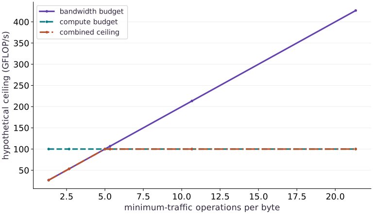
A hypothetical roofline bends at the compute budget

Predict before looking: Which square-matrix cases lie below the transition intensity?

Hypothetical bandwidth and compute ceilings with their minimum; the first two cases are bandwidth-limited. — Plot from a recorded CPU computation · JAX 0.9.2 · 1 CPU device

Read the figure

The horizontal axis is the minimum-traffic arithmetic intensity, in operations per byte. The vertical axis is a hypothetical throughput ceiling in billions of operations per second. The rising bandwidth line multiplies intensity by the assumed bandwidth; the horizontal compute line is the assumed compute budget. Neither line is a device measurement.

The combined ceiling follows the lower of these two lines. The first two cases are about $26.67$ and $53.33$ GFLOP/s; from the third matrix-size case onward the ceiling is $100$ . The change of slope occurs where the budgets meet, at intensity $5$ , which is included explicitly as an extra point between the second and third matrix-size cases.

Connect it to the computation

Each intensity comes from counting the elements in square input/output matrices and assuming one read or write per element. Increasing matrix size increases modeled reuse, so the bandwidth ceiling rises. After the compute cap is reached, further reuse cannot raise this simplified ceiling.

Actual small CPU measurements are recorded separately and include dispatch and completion waiting. Do not plot them against these invented hardware budgets as a measured efficiency claim. A real roofline study needs appropriate hardware limits and traffic evidence.

Open full-size figure Download data and provenance

The notebook contains the data experiment, plotting code, and recorded figure output. Rerun it to test your changes.

Where to put & run this code: Work in phases/08-performance/04-reason-with-hlo-and-the-roofline-model/code/main.py (or downloaded exercises/performance-04.py / exercises/performance-04.ipynb) and execute from the repository root with python3 phases/08-performance/04-reason-with-hlo-and-the-roofline-model/code/main.py.

1 Inspect a specialized lowered computation

Create a Python file in the course environment. Add this block after the preceding block, then run the assembled file.

main.py · append build step 1

# Step 1 — Inspect a specialized lowered computation: StableHLO establishes the operation and shape contract.
import time
import numpy as np
import jax
import jax.numpy as jnp

StableHLO establishes the operation and shape contract. Numerical equality is checked after compiling that same lowered program.

2 Calculate an explicitly hypothetical model

Create a Python file in the course environment. Add this block after the preceding block, then run the assembled file.

main.py · append build step 2

# Step 2 — Calculate an explicitly hypothetical model: The square-matrix simplification supplies an independent...
def workload(a,b):return jnp.tanh(a@b)
# Construct and reshape `a` into the target tensor dimensions.
a=jnp.arange(32*16,dtype=jnp.float32).reshape(32,16)/512
# Construct and reshape `b` into the target tensor dimensions.
b=jnp.arange(16*8,dtype=jnp.float32).reshape(16,8)/128
# Wrap with `jax.jit` (`lowered`) so XLA traces and compiles the function.
lowered=jax.jit(workload).lower(a,b)
# Trace or lower the function to inspect its compiler representation (`stablehlo`).
stablehlo=str(lowered.compiler_ir(dialect='stablehlo'))
assert 'dot_general' in stablehlo and 'tanh' in stablehlo
# Trace or lower the function to inspect its compiler representation (`executable`).
executable=lowered.compile()
# Convert `` to a host NumPy array for inspection or verification.
np.testing.assert_allclose(executable(a,b),np.tanh(np.asarray(a)@np.asarray(b)),rtol=2e-5,atol=2e-5)
print('StableHLO operations present: dot_general and tanh')
print('Compiler estimates (backend-specific):',executable.cost_analysis())

Code building blocks in this step

jnp.arange(n, dtype=...) — Creates a 1-D JAX array of evenly spaced values [0, 1, ..., n-1] on the target device.
array.reshape(new_shape) — Reorganizes tensor axes without changing the total element count (array.size).
jnp.allclose(actual, expected, rtol=..., atol=...) — Checks that two arrays match elementwise within floating-point tolerance.
jax.jit(fn) / @jax.jit — Traces fn with abstract shapes and compiles a fused XLA executable cached by input shape and dtype.

The square-matrix simplification supplies an independent arithmetic check. The hardware budgets are illustrative constants.

3 Keep runtime observations separate

Create a Python file in the course environment. Add this block after the preceding block, then run the assembled file.

main.py · append build step 3

# An analytic traffic model, not a measurement of this CPU.
def contract(m,k,n,itemsize=4):
    # Guard input contract (`min(m, k, n, itemsize) <= 0`) and fail fast if violated.
    if min(m,k,n,itemsize)<=0:raise ValueError('positive dimensions and itemsize required')
    flops=2*m*k*n  # conventional multiply-add count; excludes tanh
    minimum_bytes=itemsize*(m*k+k*n+m*n)
    return flops,minimum_bytes,flops/minimum_bytes
sizes=np.array([8,16,32,64,128])
intensity=np.array([contract(int(n),int(n),int(n))[2] for n in sizes])
# Execute `np.testing.assert_allclose(intensity,sizes/6)`
np.testing.assert_allclose(intensity,sizes/6)
peak=100e9
bandwidth=20e9  # hypothetical budgets, not device specifications
memory_ceiling=bandwidth*intensity
roofline=np.minimum(peak,memory_ceiling)
# Execute `np.testing.assert_allclose(roofline[:2]/1e9,[80/3,160/3])`
np.testing.assert_allclose(roofline[:2]/1e9,[80/3,160/3])
assert np.all(roofline[2:]==peak)

Code building blocks in this step

jnp.allclose(actual, expected, rtol=..., atol=...) — Checks that two arrays match elementwise within floating-point tolerance.

Warm samples measure the current CPU, while the work count remains a matmul-only convention. The code never asserts a speedup or hardware saturation.

4 Keep runtime observations separate

Create a Python file in the course environment. Add this block after the preceding block, then run the assembled file.

main.py · append build step 4

# Step 4 — Keep runtime observations separate: Warm samples measure the current CPU, while the work count remains...
executable(a,b).block_until_ready()
times=[]
for _ in range(5):
    # Synchronize host execution until asynchronous device computation completes.
    # Synchronize host execution until asynchronous device computation completes.
    # Synchronize host execution until asynchronous device computation completes.
    start=time.perf_counter()
    executable(a,b).block_until_ready()
    times.append(time.perf_counter()-start)
flops,minimum_bytes,ai=contract(32,16,8)
print('Local CPU samples seconds:',times)
print('Matmul-only accounting:',{'flops':flops,'minimum_bytes':minimum_bytes,'flops_per_byte':ai})
print('Hypothetical ceilings GFLOP/s:',(roofline/1e9).tolist())

Code building blocks in this step

jax.block_until_ready(output) — Synchronizes with the accelerator/CPU device so asynchronous dispatch finishes before wall-clock timing.

Warm samples measure the current CPU, while the work count remains a matmul-only convention. The code never asserts a speedup or hardware saturation.

View the cumulative build in main.py

These blocks append in order to the same file.

main.py · cumulative Python build

# Step 1 — Inspect a specialized lowered computation: StableHLO establishes the operation and shape contract.
import time
import numpy as np
import jax
import jax.numpy as jnp

# Step 2 — Calculate an explicitly hypothetical model: The square-matrix simplification supplies an independent...
def workload(a,b):return jnp.tanh(a@b)
# Construct and reshape `a` into the target tensor dimensions.
a=jnp.arange(32*16,dtype=jnp.float32).reshape(32,16)/512
# Construct and reshape `b` into the target tensor dimensions.
b=jnp.arange(16*8,dtype=jnp.float32).reshape(16,8)/128
# Wrap with `jax.jit` (`lowered`) so XLA traces and compiles the function.
lowered=jax.jit(workload).lower(a,b)
# Trace or lower the function to inspect its compiler representation (`stablehlo`).
stablehlo=str(lowered.compiler_ir(dialect='stablehlo'))
assert 'dot_general' in stablehlo and 'tanh' in stablehlo
# Trace or lower the function to inspect its compiler representation (`executable`).
executable=lowered.compile()
# Convert `` to a host NumPy array for inspection or verification.
np.testing.assert_allclose(executable(a,b),np.tanh(np.asarray(a)@np.asarray(b)),rtol=2e-5,atol=2e-5)
print('StableHLO operations present: dot_general and tanh')
print('Compiler estimates (backend-specific):',executable.cost_analysis())

# An analytic traffic model, not a measurement of this CPU.
def contract(m,k,n,itemsize=4):
    # Guard input contract (`min(m, k, n, itemsize) <= 0`) and fail fast if violated.
    if min(m,k,n,itemsize)<=0:raise ValueError('positive dimensions and itemsize required')
    flops=2*m*k*n  # conventional multiply-add count; excludes tanh
    minimum_bytes=itemsize*(m*k+k*n+m*n)
    return flops,minimum_bytes,flops/minimum_bytes
sizes=np.array([8,16,32,64,128])
intensity=np.array([contract(int(n),int(n),int(n))[2] for n in sizes])
# Execute `np.testing.assert_allclose(intensity,sizes/6)`
np.testing.assert_allclose(intensity,sizes/6)
peak=100e9
bandwidth=20e9  # hypothetical budgets, not device specifications
memory_ceiling=bandwidth*intensity
roofline=np.minimum(peak,memory_ceiling)
# Execute `np.testing.assert_allclose(roofline[:2]/1e9,[80/3,160/3])`
np.testing.assert_allclose(roofline[:2]/1e9,[80/3,160/3])
assert np.all(roofline[2:]==peak)

# Step 4 — Keep runtime observations separate: Warm samples measure the current CPU, while the work count remains...
executable(a,b).block_until_ready()
times=[]
for _ in range(5):
    # Synchronize host execution until asynchronous device computation completes.
    # Synchronize host execution until asynchronous device computation completes.
    # Synchronize host execution until asynchronous device computation completes.
    start=time.perf_counter()
    executable(a,b).block_until_ready()
    times.append(time.perf_counter()-start)
flops,minimum_bytes,ai=contract(32,16,8)
print('Local CPU samples seconds:',times)
print('Matmul-only accounting:',{'flops':flops,'minimum_bytes':minimum_bytes,'flops_per_byte':ai})
print('Hypothetical ceilings GFLOP/s:',(roofline/1e9).tolist())

Run the example

python3 phases/08-performance/04-reason-with-hlo-and-the-roofline-model/code/main.py

About this command

This shortcut uses an activated macOS/Linux course environment in the repository folder. For Windows, use the explicit interpreter command in “Setup help” above. The script includes worked examples and reference solutions.

Inspect the complete assembled example

main.py · complete Python example

# Step 1 — Inspect a specialized lowered computation: StableHLO establishes the operation and shape contract.
import time
import numpy as np
import jax
import jax.numpy as jnp

# Step 2 — Calculate an explicitly hypothetical model: The square-matrix simplification supplies an independent...
def workload(a,b):return jnp.tanh(a@b)
# Construct and reshape `a` into the target tensor dimensions.
a=jnp.arange(32*16,dtype=jnp.float32).reshape(32,16)/512
# Construct and reshape `b` into the target tensor dimensions.
b=jnp.arange(16*8,dtype=jnp.float32).reshape(16,8)/128
# Wrap with `jax.jit` (`lowered`) so XLA traces and compiles the function.
lowered=jax.jit(workload).lower(a,b)
# Trace or lower the function to inspect its compiler representation (`stablehlo`).
stablehlo=str(lowered.compiler_ir(dialect='stablehlo'))
assert 'dot_general' in stablehlo and 'tanh' in stablehlo
# Trace or lower the function to inspect its compiler representation (`executable`).
executable=lowered.compile()
# Convert `` to a host NumPy array for inspection or verification.
np.testing.assert_allclose(executable(a,b),np.tanh(np.asarray(a)@np.asarray(b)),rtol=2e-5,atol=2e-5)
print('StableHLO operations present: dot_general and tanh')
print('Compiler estimates (backend-specific):',executable.cost_analysis())

# An analytic traffic model, not a measurement of this CPU.
def contract(m,k,n,itemsize=4):
    # Guard input contract (`min(m, k, n, itemsize) <= 0`) and fail fast if violated.
    if min(m,k,n,itemsize)<=0:raise ValueError('positive dimensions and itemsize required')
    flops=2*m*k*n  # conventional multiply-add count; excludes tanh
    minimum_bytes=itemsize*(m*k+k*n+m*n)
    return flops,minimum_bytes,flops/minimum_bytes
sizes=np.array([8,16,32,64,128])
intensity=np.array([contract(int(n),int(n),int(n))[2] for n in sizes])
# Execute `np.testing.assert_allclose(intensity,sizes/6)`
np.testing.assert_allclose(intensity,sizes/6)
peak=100e9
bandwidth=20e9  # hypothetical budgets, not device specifications
memory_ceiling=bandwidth*intensity
roofline=np.minimum(peak,memory_ceiling)
# Execute `np.testing.assert_allclose(roofline[:2]/1e9,[80/3,160/3])`
np.testing.assert_allclose(roofline[:2]/1e9,[80/3,160/3])
assert np.all(roofline[2:]==peak)

# Step 4 — Keep runtime observations separate: Warm samples measure the current CPU, while the work count remains...
executable(a,b).block_until_ready()
times=[]
for _ in range(5):
    # Synchronize host execution until asynchronous device computation completes.
    # Synchronize host execution until asynchronous device computation completes.
    # Synchronize host execution until asynchronous device computation completes.
    start=time.perf_counter()
    executable(a,b).block_until_ready()
    times.append(time.perf_counter()-start)
flops,minimum_bytes,ai=contract(32,16,8)
print('Local CPU samples seconds:',times)
print('Matmul-only accounting:',{'flops':flops,'minimum_bytes':minimum_bytes,'flops_per_byte':ai})
print('Hypothetical ceilings GFLOP/s:',(roofline/1e9).tolist())

Expected result: StableHLO contains the declared dot and activation. The matmul accounting is $8192$ operations and $3584$ minimum bytes; the hypothetical ceilings begin near $26.67$ , $53.33$ , then $100$ GFLOP/s. CPU times vary.

Recorded reference execution

Reference output captured from executing the complete lesson script (code/main.py) and its assertions in the course CPU environment.

2026-10-20T10:47:39.421946+00:00 · Python 3.14.3 · JAX 0.9.2 · 1 CPU device

StableHLO operations present: dot_general and tanh
Compiler estimates (backend-specific): {'flops': 8192.0, 'bytes accessed1{}': 512.0, 'bytes accessedout{}': 2048.0, 'transcendentals': 256.0, 'bytes accessed': 5632.0, 'utilization1{}': 1.0, 'utilization0{}': 2.0, 'bytes accessed0{}': 3072.0}
Local CPU samples seconds: [2.1084211766719818e-05, 7.845880463719368e-05, 5.645817145705223e-05, 4.0166545659303665e-05, 3.654090687632561e-05]
Matmul-only accounting: {'flops': 8192, 'minimum_bytes': 3584, 'flops_per_byte': 2.2857142857142856}
Hypothetical ceilings GFLOP/s: [26.666666666666664, 53.33333333333333, 100.0, 100.0, 100.0]
StableHLO operations present: dot_general and tanh
Compiler estimates (backend-specific): {'utilization1{}': 1.0, 'bytes accessed0{}': 3072.0, 'utilization0{}': 2.0, 'transcendentals': 256.0, 'bytes accessedout{}': 2048.0, 'bytes accessed1{}': 512.0, 'flops': 8192.0, 'bytes accessed': 5632.0}
Local CPU samples seconds: [2.9209069907665253e-05, 2.4625100195407867e-05, 1.6333069652318954e-05, 1.2042000889778137e-05, 1.1958181858062744e-05]
Matmul-only accounting: {'flops': 8192, 'minimum_bytes': 3584, 'flops_per_byte': 2.2857142857142856}
Hypothetical ceilings GFLOP/s: [26.666666666666664, 53.33333333333333, 100.0, 100.0, 100.0]
Ceilings with twice minimum traffic GFLOP/s: [13.333333333333332, 26.666666666666664, 53.33333333333333, 100.0, 100.0]
Changed contract: 27648 8064 3.4285714285714284 bandwidth-limited in the hypothetical model
Arithmetic unchanged; modeled traffic halved and intensity doubled.
PASS: performance-04

Download execution record · The notebook includes executed cells and figure outputs. Compare your run with these values; timings depend on the machine.

Double the assumed data movement

Double the assumed data movement · Python experiment

# Experiment — Double the assumed data movement: The work is unchanged; doubling transferred bytes halves intensity.
reduced=intensity/2
revised=np.minimum(peak,bandwidth*reduced)
# Execute `np.testing.assert_allclose(revised[:2],roofline[:2]/2)`
np.testing.assert_allclose(revised[:2],roofline[:2]/2)
assert revised[-1]==peak
print('Ceilings with twice minimum traffic GFLOP/s:',(revised/1e9).tolist())

Expected: The first bandwidth-limited ceilings halve; a sufficiently intense case stays compute-limited.

The work is unchanged; doubling transferred bytes halves intensity. This is a sensitivity calculation, not a measured cache miss rate.

Hands-On Exercise · Modify & Verify Run in the declared lesson environment

Make it yours

Where to put your code: Append your solution at the bottom of phases/08-performance/04-reason-with-hlo-and-the-roofline-model/code/main.py (or inside the Make it yours cell of exercises/performance-04.ipynb) and run python3 phases/08-performance/04-reason-with-hlo-and-the-roofline-model/code/main.py to verify your prediction before opening the reference solution.

Derive the work and minimum traffic for shapes $(48,24)$ and $(24,12)$ . Compare your hand calculation with the contract function and report the hypothetical limiting budget.

Show a writing guide and starter scaffold

How to write this exercise code: step-by-step recipe & starter scaffold

1. Key functions & syntax to use:

jnp.allclose(actual, expected, rtol=..., atol=...) — Checks that two arrays match elementwise within floating-point tolerance.

2. Step-by-step implementation plan:

Execute np.testing.assert_allclose(ratio,24/7)

Starter code scaffold · copy into your file & fill in the TODOs

# Exercise solution: Derive the work and minimum traffic for shapes (48,24) and (24,12).
work,traffic,ratio = contract(...)  # TODO: compute work,traffic,ratio
assert work  # TODO: complete assertion check
# Execute `np.testing.assert_allclose(ratio,24/7)`
np.testing.assert_allclose(ratio,24/7)
assert bandwidth*ratio  # TODO: complete assertion check
print('Changed contract:',work,traffic,ratio,'bandwidth-limited in the hypothetical model')

Reveal the reference solution

Reference solution

# Exercise solution: Derive the work and minimum traffic for shapes (48,24) and (24,12).
work,traffic,ratio=contract(48,24,12)
assert work==27648 and traffic==8064
# Execute `np.testing.assert_allclose(ratio,24/7)`
np.testing.assert_allclose(ratio,24/7)
assert bandwidth*ratio<peak
print('Changed contract:',work,traffic,ratio,'bandwidth-limited in the hypothetical model')

Keep the same shapes but change storage precision

Transfer

Change only the assumed element size from four bytes to two bytes. Calculate the resulting traffic and intensity, and explain why this is insufficient to predict an actual speedup.

Show a writing guide and starter scaffold

How to write this practice solution: step-by-step recipe & starter scaffold

1. Key functions & syntax to use:

jnp.allclose(actual, expected, rtol=..., atol=...) — Checks that two arrays match elementwise within floating-point tolerance.

2. Step-by-step implementation plan:

Execute np.testing.assert_allclose(i16,2*i32)

Starter code scaffold · copy into your file & fill in the TODOs

# Keep the same shapes but change storage precision (Transfer): Changing storage bytes in an accounting model does not...
f32,b32,i32 = contract(...)  # TODO: compute f32,b32,i32
f16,b16,i16 = contract(...)  # TODO: compute f16,b16,i16
assert f32  # TODO: complete assertion check
# Execute `np.testing.assert_allclose(i16,2*i32)`
np.testing.assert_allclose(i16,2*i32)
print('Arithmetic unchanged; modeled traffic halved and intensity doubled.')

Show a hint

The model assumes both inputs and output use that element size; real accumulation and conversion may differ.

Reveal reference solution and reasoning

Keep the same shapes but change storage precision · Python solution

# Keep the same shapes but change storage precision (Transfer): Changing storage bytes in an accounting model does not...
f32,b32,i32=contract(32,16,8,4)
f16,b16,i16=contract(32,16,8,2)
assert f32==f16 and b32==2*b16
# Execute `np.testing.assert_allclose(i16,2*i32)`
np.testing.assert_allclose(i16,2*i32)
print('Arithmetic unchanged; modeled traffic halved and intensity doubled.')

Changing storage bytes in an accounting model is separate from native arithmetic support, accumulation policy, quality preservation or measured runtime improvement.

Diagnose the result

If a roofline claim looks implausible, check operation-count convention, byte units, element size, memory level and timing boundary. Inspect compiler estimates separately from measured traffic; neither should be silently relabeled as the other.

Carry forward

Lowered text describes a specialized program, not a timeline.
Arithmetic intensity depends on an explicit traffic model.
A roofline is a ceiling under assumptions, not a promised runtime.

Keep your evidence

Download evidence template

Keep StableHLO, synchronized CPU samples and independent output parity. Derive the byte/FLOP model and label the roofline peak and bandwidth as hypothetical.

Save your modified code, its output, and an explanation of your prediction. Checkpoint answers and exercise evidence are tracked separately.

Saved in this browser. Export or back up your portfolio anytime in My learning.

Save work for this lesson

Verified on local CPU. Stage to a Cloud TPU VM via Cloud TPU setup to record accelerator execution receipts (TODO: add automated Cloud TPU CI execution receipts).

Reason with HLO and the roofline model

What you will be able to do

The problem

The idea

Read a roofline as a conditional bound

Read the contract before the compiler text

Count work with a stated convention

Minimum traffic is an assumption you can challenge

Find the corner in a hypothetical roofline

Compare measurements only after checking equivalence

A hypothetical roofline bends at the compute budget

Read the figure

Connect it to the computation

1 Inspect a specialized lowered computation

2 Calculate an explicitly hypothetical model

3 Keep runtime observations separate

4 Keep runtime observations separate

Run the example

Recorded reference execution

Double the assumed data movement

Make it yours

Keep the same shapes but change storage precision

Check your understanding

Diagnose the result

Carry forward

Keep your evidence

Primary references