Core Foundation · Local CPULaptop CPULesson 5 of 12 in Phase 04

Phase 04 / Math & optimization

Gradient checking and numerical accuracy

Revision v0.7.0 · 2026-10-20

Lesson · about 80 minutes · CPU practice

Compare autodiff with finite differences over several step sizes.

Phase study guide: preparation, milestones and project evidence

Before you start

Before this: The chain rule, Jacobians, and directions
Hardware: CPU

Download notebook

Other downloads

Python worked examples Lesson text

Setup help: Python, notebook, or Cloud TPU VM

Use the tested CPU packages (the recorded environment uses Python 3.14.3). Other Python versions and accelerator environments require separate checks. The optional Cloud TPU specialization explains the target-specific execution boundaries. Logical CPU devices practice partitioning; they do not simulate TPU performance.

Download the repository ZIP or use your existing checkout. Extract it and open a terminal in the folder containing requirements-cpu.txt. The beginner ZIP is separate; these lessons use the full repository folder.

macOS / Linux terminal · repository folder

python3 -m venv .venv
source .venv/bin/activate
python -m pip install -r requirements-cpu.txt

PowerShell · repository folder

py -3 -m venv .venv
.\.venv\Scripts\python.exe -m pip install -r requirements-cpu.txt

After activation, run the complete worked example from that same folder:

macOS / Linux terminal · activated environment

python phases/04-optimization/02-gradient-checking-and-numerical-accuracy/code/main.py

PowerShell command · repository folder

.\.venv\Scripts\python.exe phases/04-optimization/02-gradient-checking-and-numerical-accuracy/code/main.py

For an incremental build, create main.py in your own practice folder, append each build block in order, and run python main.py with this environment active. Keep that file separate from the downloaded reference solution.

Download this lesson’s notebook. Open it with a Python kernel using the course environment. Run cells from the top after restarting the kernel; experiments depend on earlier definitions.

For local Jupyter, first install the course requirements using the Local Python steps, then use your environment’s Python to start Jupyter:

macOS / Linux terminal · activated course environment

python -m pip install jupyterlab
python -m jupyter lab

PowerShell command · repository folder

.\.venv\Scripts\python.exe -m pip install jupyterlab
.\.venv\Scripts\python.exe -m jupyter lab

Select the downloaded optimization-02.ipynb file in JupyterLab. The notebook contains reference solutions; make your prediction and attempt each practice task before opening them. Restart the kernel before changing logical device setup.

Check: Both gradients are approximately $[-3., 2.5]$ . The analytic and autodiff gradients agree; finite differences agree within tolerance.

Revisit the guided CPU setup · Open 19: TPU Setup. Package instructions are CPU instructions; Windows and accelerator environments need their own validation.

Phase 04.05 Stage 1 of 5 · Understand

1 Understand 2 Build & Run 3 Experiment 4 Exercise & Check 5 Evidence

What you will be able to do

Build an independent derivative estimate
Separate truncation error from cancellation
Test directions as well as coordinates
Recognize what a gradient check cannot prove
Do not mistake a kink for a smooth derivative

The problem

JAX can differentiate your loss, but how can you check the answer independently? We’ll nudge one weight a little in each direction and compare the change in loss with the reported gradient. You’ll also see why making the nudge smaller and smaller eventually hurts a floating-point calculation.

The idea

A finite difference estimates a derivative by comparing nearby function values. It gives us an independent check on autodiff, but it introduces its own approximation and floating-point errors. The perturbation must be small enough to be local and large enough to produce a resolvable difference.

Explain why a smaller perturbation can be worse

For a centered difference, evaluate the function on both sides of the point, subtract, and divide by twice the perturbation. With a quadratic, the centered formula has an exact cancellation of its truncation term in real arithmetic. That special case should not be described as a universal error curve for every smooth function.

In floating point, the two function values can become almost indistinguishable as the perturbation shrinks. Subtracting them loses useful information, and dividing by a tiny number amplifies the error. The smallest perturbation is therefore not automatically the best check.

Read the saved error plot using its logarithmic axes and actual minimum region. Keep dtype, parameter scale and tolerance together. Compare several perturbations, then use an analytic derivative where available to decide whether disagreement comes from autodiff or the numerical oracle.

Build an independent derivative estimate

Our objective is $(w_0-2)^2+(w_1+1)^2$ . At $[0.5, 0.25]$ , the derivative is $[-3, 2.5]$ . This formula comes from elementary differentiation, so it can check the automatic result without invoking another autodiff API. The function returns a scalar because grad requires a scalar output.

Central differences probe each coordinate along a basis vector: hold all other coordinates fixed, evaluate at $w+h e_i$ and $w-h e_i$ , then divide the difference by $2h$ . vmap batches these independent probes; it does not make the approximation exact. In the formula, $e_i$ is a vector with a $1$ in position $i$ and zeros elsewhere. It lets us move just one weight while keeping the others fixed. The symbol $\approx$ reminds us that this is an estimate.

\frac{\partial L}{\partial w_i}\approx\frac{L(w+h e_i)-L(w-h e_i)}{2h}

Separate truncation error from cancellation

For a general smooth function, central difference has an approximation error that typically shrinks quadratically with $h$ near a regular point. This quadratic objective is special: its central difference is exact in real arithmetic. Any discrepancy here mainly exposes floating-point effects. Do not use it alone to demonstrate a universal error curve.

Float32 cannot represent every nearby number. With an extremely small step, the two perturbed inputs can round to the same stored value. Subtracting their function values then gives zero rather than the derivative. A step sweep is evidence about this computation, not a recipe that works at every scale.

Test directions as well as coordinates

A directional derivative compares $\nabla L(w)^\mathsf{T}v$ with a finite difference along the direction vector $v$ . This is useful for large parameter trees because a few directions cost fewer evaluations than probing every scalar. It can miss an error orthogonal to all tested directions, so combine it with several points and known structural cases.

An allclose check permits absolute error near zero and relative error for larger values. Record the actual difference and dtype alongside a pass/fail result. Relaxing a tolerance until a broken calculation passes removes the value of the check.

Recognize what a gradient check cannot prove

Autodiff differentiates the supplied program. If the loss accidentally omits a feature or uses the wrong targets, a perfect derivative check of that wrong loss can still pass. Compare expected predictions and loss values first, then derivatives.

At a kink such as abs(0), a classical derivative does not exist. A symmetric finite difference can report zero while autodiff follows an implementation convention. Check smooth points on either side and document the boundary instead of treating the mismatch as automatic evidence of a JAX defect.

Do not mistake a kink for a smooth derivative

The function $f(x)=|x|$ has slope $-1$ for negative inputs and $1$ for positive inputs. There is no classical derivative at zero because the one-sided slopes disagree. A symmetric finite difference at zero nevertheless returns zero. This is a property of the probe, not a proof of differentiability. For a piecewise model, first test points that stay inside a smooth region, then document the boundary convention separately.

Smaller perturbations eventually lose accuracy

Predict before looking: Will shrinking the finite-difference step always improve the answer?

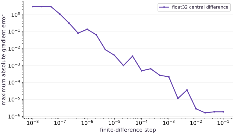
Read the figure

The horizontal axis is the finite-difference step $h$ , increasing from left to right. The vertical axis is the largest absolute discrepancy between the numerical gradient and the analytic gradient. Both axes are logarithmic: a change by one power of ten represents a tenfold change, not an equal additive increment.

At the smallest steps, the error stays near $3$ . Moving right to steps around $10^{-2}$ brings it down to a few times $10^{-6}$ , with small irregular rises along the way. All displayed errors are positive; none of the plotted estimates is exactly equal to the analytic gradient.

Connect it to the computation

At very small steps, float32 rounding makes the two nearby function evaluations indistinguishable or nearly so. Their subtraction then loses the change we are trying to measure. Dividing that damaged difference by an even smaller step does not repair it. The left-hand plateau is therefore a failure of the numerical estimate, not evidence that autodiff is wrong.

This particular objective is quadratic, so a central difference has no truncation error in exact arithmetic. Do not expect a pronounced U-shaped error curve on the right of this example. For a general nonlinear objective, overly large steps can introduce truncation error too. Check several step sizes and look for agreement across a useful range, rather than choosing the smallest available step.

Open full-size figure Download data and provenance

The notebook contains the data experiment, plotting code, and recorded figure output. Rerun it to test your changes.

Where to put & run this code: Work in phases/04-optimization/02-gradient-checking-and-numerical-accuracy/code/main.py (or downloaded exercises/optimization-02.py / exercises/optimization-02.ipynb) and execute from the repository root with python3 phases/04-optimization/02-gradient-checking-and-numerical-accuracy/code/main.py.

1 Prepare the inputs

Create a file named main.py in your activated learning environment. Add these imports and inputs first. Shapes and numeric types are part of the experiment.

main.py · append build step 1

# Step 1 — 1. Prepare the inputs: This block establishes the values used by the following steps; run...
import jax
import jax.numpy as jnp

This block establishes the values used by the following steps; run the completed file after step $3$ .

2 Define the computation

Append this block below the inputs. Before proceeding, trace which values are inputs, predictions, and state.

main.py · append build step 2

# Step 2 — 2. Define the computation: Each row of basis perturbs one coordinate.
def objective(w):
    return jnp.sum((w - jnp.array([2., -1.])) ** 2)
w = jnp.array([0.5, 0.25], dtype=jnp.float32)
h = 1e-2
basis = jnp.eye(2)
# Vectorize across the batch dimension with `jax.vmap` (`finite`).
finite = jax.vmap(lambda e: (objective(w+h*e)-objective(w-h*e))/(2*h))(basis)
# Differentiate the objective to obtain `automatic` via automatic differentiation.
automatic = jax.grad(objective)(w)
analytic = 2 * (w - jnp.array([2., -1.]))

Code building blocks in this step

jnp.array(values, dtype=...) — Constructs an immutable device-backed JAX array from Python/NumPy values.
jnp.zeros / jnp.ones(shape, dtype=...) — Allocates a tensor of the given shape initialized with constants.
x.sum(axis=...) / x.mean(axis=..., keepdims=...) — Reduces values along the named axis (the axis you name is collapsed unless keepdims=True).
jax.grad(loss_fn)(params, ...) — Transforms a scalar-output function into a function returning the gradient PyTree with the same structure as params.

Each row of basis perturbs one coordinate. vmap returns both central differences; automatic and analytic are separate references for comparison.

3 Measure and verify

Append the remaining block, then run python main.py in the terminal. Compare the printed result with the expected output below. Assertions stop execution if the contract fails.

main.py · append build step 3

# Step 3 — 3. Measure and verify: Both gradients are approximately [-3., 2.5].
print("Finite difference:", finite)
print("Autodiff:", automatic)
assert jnp.allclose(automatic, analytic)
assert jnp.allclose(finite, automatic, atol=2e-4, rtol=2e-4)

Code building blocks in this step

jnp.allclose(actual, expected, rtol=..., atol=...) — Checks that two arrays match elementwise within floating-point tolerance.

Both gradients are approximately $[-3., 2.5]$ . The analytic and autodiff gradients agree; finite differences agree within tolerance.

View the cumulative build in main.py

These blocks append in order to the same file.

main.py · cumulative Python build

# Step 1 — 1. Prepare the inputs: This block establishes the values used by the following steps; run...
import jax
import jax.numpy as jnp

# Step 2 — 2. Define the computation: Each row of basis perturbs one coordinate.
def objective(w):
    return jnp.sum((w - jnp.array([2., -1.])) ** 2)
w = jnp.array([0.5, 0.25], dtype=jnp.float32)
h = 1e-2
basis = jnp.eye(2)
# Vectorize across the batch dimension with `jax.vmap` (`finite`).
finite = jax.vmap(lambda e: (objective(w+h*e)-objective(w-h*e))/(2*h))(basis)
# Differentiate the objective to obtain `automatic` via automatic differentiation.
automatic = jax.grad(objective)(w)
analytic = 2 * (w - jnp.array([2., -1.]))

# Step 3 — 3. Measure and verify: Both gradients are approximately [-3., 2.5].
print("Finite difference:", finite)
print("Autodiff:", automatic)
assert jnp.allclose(automatic, analytic)
assert jnp.allclose(finite, automatic, atol=2e-4, rtol=2e-4)

Run the example

python3 phases/04-optimization/02-gradient-checking-and-numerical-accuracy/code/main.py

About this command

This shortcut uses an activated macOS/Linux course environment in the repository folder. For Windows, use the explicit interpreter command in “Setup help” above. The script includes worked examples and reference solutions.

Inspect the complete assembled example

main.py · complete Python example

# Step 1 — 1. Prepare the inputs: This block establishes the values used by the following steps; run...
import jax
import jax.numpy as jnp
# Step 2 — 2. Define the computation: Each row of basis perturbs one coordinate.
def objective(w):
    return jnp.sum((w - jnp.array([2., -1.])) ** 2)
w = jnp.array([0.5, 0.25], dtype=jnp.float32)
h = 1e-2
basis = jnp.eye(2)
# Vectorize across the batch dimension with `jax.vmap` (`finite`).
finite = jax.vmap(lambda e: (objective(w+h*e)-objective(w-h*e))/(2*h))(basis)
# Differentiate the objective to obtain `automatic` via automatic differentiation.
automatic = jax.grad(objective)(w)
analytic = 2 * (w - jnp.array([2., -1.]))
# Step 3 — 3. Measure and verify: Both gradients are approximately [-3., 2.5].
print("Finite difference:", finite)
print("Autodiff:", automatic)
assert jnp.allclose(automatic, analytic)
assert jnp.allclose(finite, automatic, atol=2e-4, rtol=2e-4)

Expected result: Both gradients are approximately $[-3., 2.5]$ . The analytic and autodiff gradients agree; finite differences agree within tolerance.

Recorded reference execution

Reference output captured from executing the complete lesson script (code/main.py) and its assertions in the course CPU environment.

2026-10-20T10:45:42.659689+00:00 · Python 3.14.3 · JAX 0.9.2 · 1 CPU device

Finite difference: [-2.9999971  2.4999976]
Autodiff: [-3.   2.5]
Finite difference: [-2.9999971  2.4999976]
Autodiff: [-3.   2.5]
h / max error: 0.1 1.9073486328125e-06
h / max error: 0.01 2.86102294921875e-06
h / max error: 0.0001 0.0004978179931640625
h / max error: 1e-08 3.0
PASS: optimization-02

Download execution record · The notebook includes executed cells and figure outputs. Compare your run with these values; timings depend on the machine.

Sweep the perturbation size

Sweep the perturbation size · Python experiment

# Experiment — Sweep the perturbation size: Nearby float32 inputs can coincide, so reducing the step does...
for step_size in [1e-1, 1e-2, 1e-4, 1e-8]:
    # Vectorize across the batch dimension with `jax.vmap` (`estimate`).
    estimate = jax.vmap(lambda e: (objective(w+step_size*e)-objective(w-step_size*e))/(2*step_size))(basis)
    print("h / max error:", step_size, float(jnp.max(jnp.abs(estimate-analytic))))
# Vectorize across the batch dimension with `jax.vmap` (`tiny`).
tiny = jax.vmap(lambda e: (objective(w+1e-8*e)-objective(w-1e-8*e))/(2e-8))(basis)
assert not jnp.allclose(tiny, analytic, atol=1e-3)

Expected: The tiny-step check fails; exact intermediate errors depend on backend arithmetic.

Nearby float32 inputs can coincide, so reducing the step does not monotonically improve a check.

Check a new direction

Check a new direction · Python experiment

# Experiment — Check a new direction: A new projection supplies a separate numerical check, though it...
direction = jnp.array([1., -2.])
directional = (objective(w+h*direction)-objective(w-h*direction))/(2*h)
assert jnp.allclose(directional, -8., atol=2e-4)
assert jnp.allclose(jnp.dot(automatic, direction), -8.)

Expected: Directional derivative $-8$ within tolerance.

A new projection supplies a separate numerical check, though it does not test every direction.

A symmetric probe can hide a kink

A symmetric probe can hide a kink · Python experiment

# Experiment — A symmetric probe can hide a kink: Agreement with one numerical probe can conceal nondifferentiability.
h_kink = 0.01
symmetric = (jnp.abs(h_kink)-jnp.abs(-h_kink))/(2*h_kink)
left = (jnp.abs(0.)-jnp.abs(-h_kink))/h_kink
right = (jnp.abs(h_kink)-jnp.abs(0.))/h_kink
assert jnp.allclose(symmetric,0.)
assert jnp.allclose(left,-1.) and jnp.allclose(right,1.)
assert jnp.allclose(jax.grad(jnp.abs)(jnp.array(-2.)),-1.)
assert jnp.allclose(jax.grad(jnp.abs)(jnp.array(2.)),1.)

Expected: The symmetric estimate is $0$ ; left and right slopes are $-1$ and $1$ .

Agreement with one numerical probe can conceal nondifferentiability. Choose probes that test the assumption your claim needs.

Hands-On Exercise · Modify & Verify Run in the declared lesson environment

Make it yours

Where to put your code: Append your solution at the bottom of phases/04-optimization/02-gradient-checking-and-numerical-accuracy/code/main.py (or inside the Make it yours cell of exercises/optimization-02.ipynb) and run python3 phases/04-optimization/02-gradient-checking-and-numerical-accuracy/code/main.py to verify your prediction before opening the reference solution.

Check the gradient again at $w=[2., -1.]$ . Explain why this checks a minimum but does not prove correctness everywhere.

Show a writing guide and starter scaffold

How to write this exercise code: step-by-step recipe & starter scaffold

1. Key functions & syntax to use:

jnp.array(values, dtype=...) — Constructs an immutable device-backed JAX array from Python/NumPy values.
jnp.zeros / jnp.ones(shape, dtype=...) — Allocates a tensor of the given shape initialized with constants.
jnp.allclose(actual, expected, rtol=..., atol=...) — Checks that two arrays match elementwise within floating-point tolerance.
jax.grad(loss_fn)(params, ...) — Transforms a scalar-output function into a function returning the gradient PyTree with the same structure as params.

2. Step-by-step implementation plan:

Set up the changed input or configuration parameters requested in the prompt.
Run the target function or transformation and assert that the output matches your prediction.

Starter code scaffold · copy into your file & fill in the TODOs

# Exercise solution: Check the gradient again at w=[2., -1.].
minimum = jnp.array(...)  # TODO: compute minimum
assert jnp.allclose(jax.grad(objective)(minimum), jnp.zeros(2))  # TODO: complete assertion check
assert jnp.allclose(objective(minimum), 0.)  # TODO: complete assertion check

Reveal the reference solution

Reference solution

# Exercise solution: Check the gradient again at w=[2., -1.].
minimum = jnp.array([2., -1.])
assert jnp.allclose(jax.grad(objective)(minimum), jnp.zeros(2))
assert jnp.allclose(objective(minimum), 0.)

Move to a different smooth objective

Transfer / diagnosis

Check the derivative of sum(sin(z)) at $[0.2, -0.7]$ using cosine and central differences.

Show a writing guide and starter scaffold

How to write this practice solution: step-by-step recipe & starter scaffold

1. Key functions & syntax to use:

jnp.array(values, dtype=...) — Constructs an immutable device-backed JAX array from Python/NumPy values.
jnp.zeros / jnp.ones(shape, dtype=...) — Allocates a tensor of the given shape initialized with constants.
x.sum(axis=...) / x.mean(axis=..., keepdims=...) — Reduces values along the named axis (the axis you name is collapsed unless keepdims=True).
jnp.allclose(actual, expected, rtol=..., atol=...) — Checks that two arrays match elementwise within floating-point tolerance.

2. Step-by-step implementation plan:

Vectorize across the batch dimension with jax.vmap (fd).

Starter code scaffold · copy into your file & fill in the TODOs

# Move to a different smooth objective (Transfer / diagnosis): The analytic reference checks a nonquadratic function at a...
z = jnp.array(...)  # TODO: compute z
def trig_loss(z):
    return ...  # TODO: return computed result
# Vectorize across the batch dimension with `jax.vmap` (`fd`).
fd = jax.vmap(...)  # TODO: compute fd
assert jnp.allclose(jax.grad(trig_loss)(z), jnp.cos(z))  # TODO: complete assertion check
assert jnp.allclose(fd, jnp.cos(z), atol=5e-5, rtol=5e-5)  # TODO: complete assertion check

Show a hint

Use cosine as the analytic reference; here truncation error also matters.

Reveal reference solution and reasoning

Move to a different smooth objective · Python solution

# Move to a different smooth objective (Transfer / diagnosis): The analytic reference checks a nonquadratic function at a...
z = jnp.array([0.2, -0.7])
def trig_loss(z):
    return jnp.sum(jnp.sin(z))
# Vectorize across the batch dimension with `jax.vmap` (`fd`).
fd = jax.vmap(lambda e: (trig_loss(z+1e-2*e)-trig_loss(z-1e-2*e))/(2e-2))(jnp.eye(2))
assert jnp.allclose(jax.grad(trig_loss)(z), jnp.cos(z))
assert jnp.allclose(fd, jnp.cos(z), atol=5e-5, rtol=5e-5)

The analytic reference checks a nonquadratic function at a new point.

Catch the wrong objective despite correct gradients

Transfer / diagnosis

A model is meant to use both coordinates. Show that an objective omitting the second coordinate has a correct derivative for itself but fails the intended analytic reference. Repair it.

Show a writing guide and starter scaffold

How to write this practice solution: step-by-step recipe & starter scaffold

1. Key functions & syntax to use:

jnp.array(values, dtype=...) — Constructs an immutable device-backed JAX array from Python/NumPy values.
jnp.allclose(actual, expected, rtol=..., atol=...) — Checks that two arrays match elementwise within floating-point tolerance.
jax.grad(loss_fn)(params, ...) — Transforms a scalar-output function into a function returning the gradient PyTree with the same structure as params.

2. Step-by-step implementation plan:

Differentiate the objective to obtain bad via automatic differentiation.

Starter code scaffold · copy into your file & fill in the TODOs

# Catch the wrong objective despite correct gradients (Transfer / diagnosis): The omitted term is a specification error; numerical...
def incomplete(z):
    return ...  # TODO: return computed result
# Differentiate the objective to obtain `bad` via automatic differentiation.
bad = jax.grad(...)  # TODO: compute bad
assert jnp.allclose(bad, jnp.array([-3., 0.]))  # TODO: complete assertion check
assert not jnp.allclose(bad, analytic)  # TODO: complete assertion check
assert jnp.allclose(jax.grad(objective)(w), analytic)  # TODO: complete assertion check

Show a hint

Differentiate $(z_0-2)^2$ and compare both coordinates.

Reveal reference solution and reasoning

Catch the wrong objective despite correct gradients · Python solution

# Catch the wrong objective despite correct gradients (Transfer / diagnosis): The omitted term is a specification error; numerical...
def incomplete(z):
    return (z[0]-2.)**2
# Differentiate the objective to obtain `bad` via automatic differentiation.
bad = jax.grad(incomplete)(w)
assert jnp.allclose(bad, jnp.array([-3., 0.]))
assert not jnp.allclose(bad, analytic)
assert jnp.allclose(jax.grad(objective)(w), analytic)

The omitted term is a specification error; numerical differentiation of the same incomplete loss would not expose it.

Diagnose the result

If the finite-difference check fails, sweep several step sizes before changing the model. Inspect dtype, reduction axes, and whether the point crosses a nonsmooth operation.

Carry forward

Nearby float32 inputs can coincide, so reducing the step does not monotonically improve a check.
A new projection supplies a separate numerical check, though it does not test every direction.

Keep your evidence

Download evidence template

Save analytic and numerical derivatives, the step-size/error table with dtype, the nonquadratic transfer check, and the omitted-term failure/repair. Add the one-sided slopes showing why a symmetric probe cannot certify differentiability at a kink.

Save your modified code, its output, and an explanation of your prediction. Checkpoint answers and exercise evidence are tracked separately.

Saved in this browser. Export or back up your portfolio anytime in My learning.

Save work for this lesson

Verified on local CPU. Stage to a Cloud TPU VM via Cloud TPU setup to record accelerator execution receipts (TODO: add automated Cloud TPU CI execution receipts).

Gradient checking and numerical accuracy

What you will be able to do

The problem

The idea

Explain why a smaller perturbation can be worse

Build an independent derivative estimate

Separate truncation error from cancellation

Test directions as well as coordinates

Recognize what a gradient check cannot prove

Do not mistake a kink for a smooth derivative

Smaller perturbations eventually lose accuracy

Read the figure

Connect it to the computation

1 Prepare the inputs

2 Define the computation

3 Measure and verify

Run the example

Recorded reference execution

Sweep the perturbation size

Check a new direction

A symmetric probe can hide a kink

Make it yours

Move to a different smooth objective

Catch the wrong objective despite correct gradients

Check your understanding

Diagnose the result

Carry forward

Keep your evidence

Primary references