Core Foundation · Local CPULaptop CPULesson 9 of 12 in Phase 04

Phase 04 / Math & optimization

Regularization and honest validation

Revision v0.7.0 · 2026-10-20

Lesson · about 75 minutes · CPU practice

Derive a ridge solution, distinguish data loss from penalized loss, and select a penalty using held-out data.

Phase study guide: preparation, milestones and project evidence

Before you start

Before this: Probability, likelihood, and stable losses
Hardware: CPU

Download notebook

Other downloads

Python worked examples Lesson text

Setup help: Python, notebook, or Cloud TPU VM

Use the tested CPU packages (the recorded environment uses Python 3.14.3). Other Python versions and accelerator environments require separate checks. The optional Cloud TPU specialization explains the target-specific execution boundaries. Logical CPU devices practice partitioning; they do not simulate TPU performance.

Download the repository ZIP or use your existing checkout. Extract it and open a terminal in the folder containing requirements-cpu.txt. The beginner ZIP is separate; these lessons use the full repository folder.

macOS / Linux terminal · repository folder

python3 -m venv .venv
source .venv/bin/activate
python -m pip install -r requirements-cpu.txt

PowerShell · repository folder

py -3 -m venv .venv
.\.venv\Scripts\python.exe -m pip install -r requirements-cpu.txt

After activation, run the complete worked example from that same folder:

macOS / Linux terminal · activated environment

python phases/04-optimization/10-regularization-and-validation/code/main.py

PowerShell command · repository folder

.\.venv\Scripts\python.exe phases/04-optimization/10-regularization-and-validation/code/main.py

For an incremental build, create main.py in your own practice folder, append each build block in order, and run python main.py with this environment active. Keep that file separate from the downloaded reference solution.

Download this lesson’s notebook. Open it with a Python kernel using the course environment. Run cells from the top after restarting the kernel; experiments depend on earlier definitions.

For local Jupyter, first install the course requirements using the Local Python steps, then use your environment’s Python to start Jupyter:

macOS / Linux terminal · activated course environment

python -m pip install jupyterlab
python -m jupyter lab

PowerShell command · repository folder

.\.venv\Scripts\python.exe -m pip install jupyterlab
.\.venv\Scripts\python.exe -m jupyter lab

Select the downloaded optimization-10.ipynb file in JupyterLab. The notebook contains reference solutions; make your prediction and attempt each practice task before opening them. Restart the kernel before changing logical device setup.

Check: The regularized slope is $2$ ; data loss and penalized objective are reported separately.

Revisit the guided CPU setup · Open 19: TPU Setup. Package instructions are CPU instructions; Windows and accelerator environments need their own validation.

Phase 04.09 Stage 1 of 5 · Understand

1 Understand 2 Build & Run 3 Experiment 4 Exercise & Check 5 Evidence

What you will be able to do

Derive a ridge solution, distinguish data loss from penalized loss, and select a penalty using held-out data.
State the exact objective
Work through shrinkage by hand
Keep fitting, choosing and reporting separate
Choose which parameters to penalize

The problem

A model can fit the training data closely and still make poor predictions on new data. Can we trade a little training fit for a simpler model? We will make that tradeoff visible with a dataset small enough to solve by hand, while keeping the validation data separate from fitting.

The idea

Regularization changes which solutions training prefers. Validation helps choose settings using data that did not fit the model, and a final test estimates performance after those choices are fixed. Keeping these jobs separate makes the reported result interpretable.

Give each split one job

Imagine trying several penalty strengths. For each setting, fit weights on the training split, then score the frozen result on validation. Pick a setting using those validation results. Repeatedly using test performance to make that choice quietly turns the test into another validation set.

Preprocessing belongs inside the same boundary: fit means, scales and feature selection using training data only. Applying a transformation to validation is allowed; allowing validation to choose the transformation's fitted statistics changes the experiment.

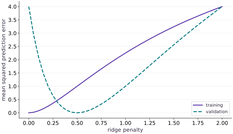
The regularization plot may show training error improving while validation error worsens. That gap motivates model selection, but one small fixture does not prove a universal best penalty. Preserve split identities and the selection rule so another person can reconstruct the decision.

State the exact objective

Let $n$ be the training sample count and $\lambda\ge0$ the penalty strength. We use mean squared error plus $\lambda\|w\|_2^2$ , without a factor of one half. Differentiating gives $2X^\mathsf{T}(Xw-y)/n+2\lambda w$ . Setting it to zero gives the linear system below. Other conventions change the numerical meaning of the same penalty value, so copy the objective along with a reported hyperparameter.

L_\lambda(w)=\frac1n\|Xw-y\|_2^2+\lambda\|w\|_2^2,\qquad (X^\mathsf{T}X+n\lambda I)w=X^\mathsf{T}y

Work through shrinkage by hand

Train a slope without a bias on inputs $(-1,1)$ and targets $(-3,3)$ . The data loss is $(w-3)^2$ , so the ridge solution is $w=3/(1+\lambda)$ . At $\lambda=0$ , it fits the training slope $3$ . At $\lambda=1/2$ , it gives slope $2$ . Our deliberately constructed validation targets follow slope $2$ , making the tradeoff easy to inspect. Real validation curves are noisier and do not guarantee that positive regularization helps.

Keep fitting, choosing and reporting separate

Fit weights on training examples for each candidate $\lambda$ . Choose using validation prediction loss, not the training objective with its penalty. Validation targets must never enter the fit or preprocessing statistics. After many choices, validation itself can be overfit; a final untouched test set estimates the selected procedure. This tiny exercise has a training and validation split only, so its result is a demonstration, not a final generalization estimate.

Choose which parameters to penalize

A bias can represent the overall target level, so many models exclude it from weight regularization. For an augmented parameter vector $(w,b)$ , use a diagonal penalty mask with entries $(1,0)$ . Scaling a feature also changes the size of its coefficient, and therefore the penalty. Standardize using training statistics when that matches your modeling choice, then reuse those statistics unchanged for validation and inference. Ridge adds curvature in penalized directions; it cannot repair leaked data or a wrong target.

Training error and validation error select different penalties

Predict before looking: Does the smallest training error imply the best validation result?

Read the figure

The horizontal axis varies the ridge penalty $\lambda$ . For each penalty, the model is fitted again. The vertical axis shows mean squared prediction error on training and validation data; it does not include the penalty term.

At $\lambda=0$ , training error is zero and validation error is $4$ . At $\lambda=0.5$ , training error rises to $1$ , but validation error falls to zero. Increasing the penalty to $2$ makes both errors $4$ . The validation curve therefore has a minimum between the extremes.

Connect it to the computation

The fitted weight is $w=3/(1+\lambda)$ . The training targets favor slope $3$ , while the validation targets in this constructed example favor slope $2$ . Moderate shrinkage moves the model toward the validation relationship; too much shrinkage moves it past that relationship and toward underfitting.

Select the penalty using the validation minimum, not the intersection of the curves or the smallest training error. Here that choice is $0.5$ . A zero validation error is a property of this tiny synthetic example, not a promise that regularization removes all error on real data.

Open full-size figure Download data and provenance

The notebook contains the data experiment, plotting code, and recorded figure output. Rerun it to test your changes.

Where to put & run this code: Work in phases/04-optimization/10-regularization-and-validation/code/main.py (or downloaded exercises/optimization-10.py / exercises/optimization-10.ipynb) and execute from the repository root with python3 phases/04-optimization/10-regularization-and-validation/code/main.py.

1 Create separate training and validation examples

Create main.py. Keep validation arrays separate from the solver inputs.

main.py · append build step 1

# Step 1 — Create separate training and validation examples: The helper solves the explicitly stated mean-loss convention.
import jax
import jax.numpy as jnp
X = jnp.array([[-1.0], [1.0]])
y = jnp.array([-3.0, 3.0])
Xv = jnp.array([[-2.0], [2.0]])
yv = jnp.array([-4.0, 4.0])

def ridge(X, y, lam):
    return jnp.linalg.solve(X.T @ X + X.shape[0] * lam * jnp.eye(X.shape[1]), X.T @ y)

def mse(w, X, y):
    return jnp.mean((X @ w - y) ** 2)

Code building blocks in this step

jnp.array(values, dtype=...) — Constructs an immutable device-backed JAX array from Python/NumPy values.
jnp.zeros / jnp.ones(shape, dtype=...) — Allocates a tensor of the given shape initialized with constants.
x.sum(axis=...) / x.mean(axis=..., keepdims=...) — Reduces values along the named axis (the axis you name is collapsed unless keepdims=True).

The helper solves the explicitly stated mean-loss convention. We use a small well-conditioned system here; this is not a general replacement for robust least-squares algorithms.

2 Verify the penalized optimum

Append the hand solution and its gradient check.

main.py · append build step 2

# Step 2 — Verify the penalized optimum: The data gradient and penalty gradient cancel at w=2.
lam = 0.5
w = ridge(X, y, lam)
objective = lambda w: mse(w, X, y) + lam * jnp.dot(w, w)
assert jnp.allclose(w, jnp.array([2.0]), atol=1e-06)
assert jnp.allclose(jax.grad(objective)(w), jnp.zeros(1), atol=1e-06)

Code building blocks in this step

jnp.array(values, dtype=...) — Constructs an immutable device-backed JAX array from Python/NumPy values.
jnp.zeros / jnp.ones(shape, dtype=...) — Allocates a tensor of the given shape initialized with constants.
jnp.allclose(actual, expected, rtol=..., atol=...) — Checks that two arrays match elementwise within floating-point tolerance.
jax.grad(loss_fn)(params, ...) — Transforms a scalar-output function into a function returning the gradient PyTree with the same structure as params.

The data gradient and penalty gradient cancel at $w=2$ .

3 Separate the quantities you report

Append the three losses and run python main.py.

main.py · append build step 3

# Step 3 — Separate the quantities you report: Training prediction loss is 1, validation loss is 0, and the...
train = mse(w, X, y)
validation = mse(w, Xv, yv)
penalized = objective(w)
assert jnp.allclose(jnp.array([train, validation, penalized]), jnp.array([1.0, 0.0, 3.0]))
print('train / validation / objective:', train, validation, penalized)

Code building blocks in this step

jnp.array(values, dtype=...) — Constructs an immutable device-backed JAX array from Python/NumPy values.
jnp.allclose(actual, expected, rtol=..., atol=...) — Checks that two arrays match elementwise within floating-point tolerance.

Training prediction loss is $1$ , validation loss is $0$ , and the penalized objective is $3$ . They answer different questions.

View the cumulative build in main.py

These blocks append in order to the same file.

main.py · cumulative Python build

# Step 1 — Create separate training and validation examples: The helper solves the explicitly stated mean-loss convention.
import jax
import jax.numpy as jnp
X = jnp.array([[-1.0], [1.0]])
y = jnp.array([-3.0, 3.0])
Xv = jnp.array([[-2.0], [2.0]])
yv = jnp.array([-4.0, 4.0])

def ridge(X, y, lam):
    return jnp.linalg.solve(X.T @ X + X.shape[0] * lam * jnp.eye(X.shape[1]), X.T @ y)

def mse(w, X, y):
    return jnp.mean((X @ w - y) ** 2)

# Step 2 — Verify the penalized optimum: The data gradient and penalty gradient cancel at w=2.
lam = 0.5
w = ridge(X, y, lam)
objective = lambda w: mse(w, X, y) + lam * jnp.dot(w, w)
assert jnp.allclose(w, jnp.array([2.0]), atol=1e-06)
assert jnp.allclose(jax.grad(objective)(w), jnp.zeros(1), atol=1e-06)

# Step 3 — Separate the quantities you report: Training prediction loss is 1, validation loss is 0, and the...
train = mse(w, X, y)
validation = mse(w, Xv, yv)
penalized = objective(w)
assert jnp.allclose(jnp.array([train, validation, penalized]), jnp.array([1.0, 0.0, 3.0]))
print('train / validation / objective:', train, validation, penalized)

Run the example

python3 phases/04-optimization/10-regularization-and-validation/code/main.py

About this command

This shortcut uses an activated macOS/Linux course environment in the repository folder. For Windows, use the explicit interpreter command in “Setup help” above. The script includes worked examples and reference solutions.

Inspect the complete assembled example

main.py · complete Python example

# Step 1 — Create separate training and validation examples: The helper solves the explicitly stated mean-loss convention.
import jax
import jax.numpy as jnp
X = jnp.array([[-1.0], [1.0]])
y = jnp.array([-3.0, 3.0])
Xv = jnp.array([[-2.0], [2.0]])
yv = jnp.array([-4.0, 4.0])

def ridge(X, y, lam):
    return jnp.linalg.solve(X.T @ X + X.shape[0] * lam * jnp.eye(X.shape[1]), X.T @ y)

def mse(w, X, y):
    return jnp.mean((X @ w - y) ** 2)

# Step 2 — Verify the penalized optimum: The data gradient and penalty gradient cancel at w=2.
lam = 0.5
w = ridge(X, y, lam)
objective = lambda w: mse(w, X, y) + lam * jnp.dot(w, w)
assert jnp.allclose(w, jnp.array([2.0]), atol=1e-06)
assert jnp.allclose(jax.grad(objective)(w), jnp.zeros(1), atol=1e-06)

# Step 3 — Separate the quantities you report: Training prediction loss is 1, validation loss is 0, and the...
train = mse(w, X, y)
validation = mse(w, Xv, yv)
penalized = objective(w)
assert jnp.allclose(jnp.array([train, validation, penalized]), jnp.array([1.0, 0.0, 3.0]))
print('train / validation / objective:', train, validation, penalized)

Expected result: The regularized slope is $2$ ; data loss and penalized objective are reported separately.

Recorded reference execution

Reference output captured from executing the complete lesson script (code/main.py) and its assertions in the course CPU environment.

2026-10-20T10:45:55.153882+00:00 · Python 3.14.3 · JAX 0.9.2 · 1 CPU device

train / validation / objective: 1.0 0.0 3.0
train / validation / objective: 1.0 0.0 3.0
penalty / train / validation: [0.  0.5 2. ] [0. 1. 4.] [4. 0. 4.]
PASS: optimization-10

Download execution record · The notebook includes executed cells and figure outputs. Compare your run with these values; timings depend on the machine.

Sweep the penalty

Sweep the penalty · Python experiment

# Experiment — Sweep the penalty: Regularization deliberately trades training fit against a...
candidates = jnp.array([0.0, 0.5, 2.0])
# Combine or mask array elements to form `fits`.
fits = jnp.stack([ridge(X, y, float(a)) for a in candidates])
training = jnp.array([mse(a, X, y) for a in fits])
validation = jnp.array([mse(a, Xv, yv) for a in fits])
assert jnp.allclose(fits[:, 0], jnp.array([3.0, 2.0, 1.0]))
assert jnp.allclose(training, jnp.array([0.0, 1.0, 4.0]))
assert jnp.allclose(validation, jnp.array([4.0, 0.0, 4.0]))
assert int(jnp.argmin(training)) != int(jnp.argmin(validation))
print('penalty / train / validation:', candidates, training, validation)

Expected: Validation selects $\lambda=0.5$ ; training error prefers $\lambda=0$ .

Regularization deliberately trades training fit against a preference for smaller weights.

Duplicate the training set

Duplicate the training set · Python experiment

# Experiment — Duplicate the training set: Using a mean data loss keeps the penalty tradeoff unchanged...
repeat = ridge(jnp.tile(X, (2, 1)), jnp.tile(y, 2), lam)
assert jnp.allclose(repeat, w, atol=1e-06)

Expected: The weights stay fixed.

Using a mean data loss keeps the penalty tradeoff unchanged under exact dataset duplication.

Hands-On Exercise · Modify & Verify Run in the declared lesson environment

Make it yours

Where to put your code: Append your solution at the bottom of phases/04-optimization/10-regularization-and-validation/code/main.py (or inside the Make it yours cell of exercises/optimization-10.ipynb) and run python3 phases/04-optimization/10-regularization-and-validation/code/main.py to verify your prediction before opening the reference solution.

For a target slope of $4$ and penalty $\lambda=1$ , derive the fitted slope and verify its gradient.

Show a writing guide and starter scaffold

How to write this exercise code: step-by-step recipe & starter scaffold

1. Key functions & syntax to use:

jnp.array(values, dtype=...) — Constructs an immutable device-backed JAX array from Python/NumPy values.
jnp.zeros / jnp.ones(shape, dtype=...) — Allocates a tensor of the given shape initialized with constants.
jnp.allclose(actual, expected, rtol=..., atol=...) — Checks that two arrays match elementwise within floating-point tolerance.
jax.grad(loss_fn)(params, ...) — Transforms a scalar-output function into a function returning the gradient PyTree with the same structure as params.

2. Step-by-step implementation plan:

Set up the changed input or configuration parameters requested in the prompt.
Run the target function or transformation and assert that the output matches your prediction.

Starter code scaffold · copy into your file & fill in the TODOs

# Exercise solution: For a target slope of 4 and penalty \lambda=1, derive the fitted slope...
y4 = jnp.array(...)  # TODO: compute y4
w4 = ridge(...)  # TODO: compute w4
assert jnp.allclose(w4, jnp.array([2.0]))  # TODO: complete assertion check
assert jnp.allclose(jax.grad(lambda z: mse(z, X, y4) + jnp.dot(z, z))(w4), jnp.zeros(1), atol=1e-06)  # TODO: complete assertion check

Reveal the reference solution

Reference solution

# Exercise solution: For a target slope of 4 and penalty \lambda=1, derive the fitted slope...
y4 = jnp.array([-4.0, 4.0])
w4 = ridge(X, y4, 1.0)
assert jnp.allclose(w4, jnp.array([2.0]))
assert jnp.allclose(jax.grad(lambda z: mse(z, X, y4) + jnp.dot(z, z))(w4), jnp.zeros(1), atol=1e-06)

Do not accidentally shrink the intercept

Transfer / diagnosis

Fit constant targets $(5,5,5)$ using inputs $(-1,0,1)$ and a bias. Compare penalizing only the slope with penalizing both parameters at $\lambda=1$ .

Show a writing guide and starter scaffold

How to write this practice solution: step-by-step recipe & starter scaffold

1. Key functions & syntax to use:

jnp.array(values, dtype=...) — Constructs an immutable device-backed JAX array from Python/NumPy values.
jnp.zeros / jnp.ones(shape, dtype=...) — Allocates a tensor of the given shape initialized with constants.
jnp.allclose(actual, expected, rtol=..., atol=...) — Checks that two arrays match elementwise within floating-point tolerance.

2. Step-by-step implementation plan:

Set up the changed input or configuration parameters requested in the prompt.
Run the target function or transformation and assert that the output matches your prediction.

Starter code scaffold · copy into your file & fill in the TODOs

# Do not accidentally shrink the intercept (Transfer / diagnosis): The mask expresses a modeling choice: shrink feature effects...
x = jnp.array(...)  # TODO: compute x
A = jnp.stack(...)  # TODO: compute A
target = jnp.full(...)  # TODO: compute target
mask = jnp.diag(...)  # TODO: compute mask
correct = jnp.linalg.solve(...)  # TODO: compute correct
all_penalized = ridge(...)  # TODO: compute all_penalized
assert jnp.allclose(correct, jnp.array([0.0, 5.0]))  # TODO: complete assertion check
assert jnp.allclose(all_penalized, jnp.array([0.0, 2.5]))  # TODO: complete assertion check

Show a hint

Use a diagonal mask $\operatorname{diag}(1,0)$ .

Reveal reference solution and reasoning

Do not accidentally shrink the intercept · Python solution

# Do not accidentally shrink the intercept (Transfer / diagnosis): The mask expresses a modeling choice: shrink feature effects...
x = jnp.array([-1.0, 0.0, 1.0])
A = jnp.stack([x, jnp.ones_like(x)], axis=1)
target = jnp.full((3,), 5.0)
mask = jnp.diag(jnp.array([1.0, 0.0]))
correct = jnp.linalg.solve(A.T @ A + 3 * mask, A.T @ target)
all_penalized = ridge(A, target, 1.0)
assert jnp.allclose(correct, jnp.array([0.0, 5.0]))
assert jnp.allclose(all_penalized, jnp.array([0.0, 2.5]))

The mask expresses a modeling choice: shrink feature effects while preserving the constant target level.

Catch preprocessing leakage

Transfer / diagnosis

Training inputs are $(0,2)$ and validation input is $100$ . Compare training-only centering with centering all inputs together. Which can be reused for a truly unseen example?

Show a writing guide and starter scaffold

How to write this practice solution: step-by-step recipe & starter scaffold

1. Key functions & syntax to use:

jnp.array(values, dtype=...) — Constructs an immutable device-backed JAX array from Python/NumPy values.
x.sum(axis=...) / x.mean(axis=..., keepdims=...) — Reduces values along the named axis (the axis you name is collapsed unless keepdims=True).
jnp.allclose(actual, expected, rtol=..., atol=...) — Checks that two arrays match elementwise within floating-point tolerance.

2. Step-by-step implementation plan:

Aggregate array values to compute train_mean.
Aggregate array values to compute leaked_mean.

Starter code scaffold · copy into your file & fill in the TODOs

# Catch preprocessing leakage (Transfer / diagnosis): Validation data must not influence fitted preprocessing.
train_x = jnp.array(...)  # TODO: compute train_x
val_x = jnp.array(...)  # TODO: compute val_x
# Aggregate array values to compute `train_mean`.
train_mean = jnp.mean(...)  # TODO: compute train_mean
# Aggregate array values to compute `leaked_mean`.
leaked_mean = jnp.mean(...)  # TODO: compute leaked_mean
assert jnp.allclose(val_x - train_mean, jnp.array([99.0]))  # TODO: complete assertion check
assert not jnp.allclose(train_mean, leaked_mean)  # TODO: complete assertion check
assert jnp.allclose(jnp.mean(train_x - train_mean), 0.0)  # TODO: complete assertion check

Show a hint

Fit the mean on training data; do not refit it on validation data.

Reveal reference solution and reasoning

Catch preprocessing leakage · Python solution

# Catch preprocessing leakage (Transfer / diagnosis): Validation data must not influence fitted preprocessing.
train_x = jnp.array([0.0, 2.0])
val_x = jnp.array([100.0])
# Aggregate array values to compute `train_mean`.
train_mean = jnp.mean(train_x)
# Aggregate array values to compute `leaked_mean`.
leaked_mean = jnp.mean(jnp.concatenate([train_x, val_x]))
assert jnp.allclose(val_x - train_mean, jnp.array([99.0]))
assert not jnp.allclose(train_mean, leaked_mean)
assert jnp.allclose(jnp.mean(train_x - train_mean), 0.0)

Validation data must not influence fitted preprocessing. Reusing training statistics preserves the meaning of held-out evaluation.

Diagnose the result

If increasing $\lambda$ improves the penalized objective but worsens predictions, check which quantity is being compared. Inspect the mean-versus-sum convention, bias mask, feature units and where preprocessing statistics were fitted.

Carry forward

Regularization deliberately trades training fit against a preference for smaller weights.
Using a mean data loss keeps the penalty tradeoff unchanged under exact dataset duplication.

Keep your evidence

Download evidence template

Keep the ridge gradient/solve comparison, penalty sweep with separate train/validation losses, duplication check and bias-mask repair.

Save your modified code, its output, and an explanation of your prediction. Checkpoint answers and exercise evidence are tracked separately.

Saved in this browser. Export or back up your portfolio anytime in My learning.

Save work for this lesson

Verified on local CPU. Stage to a Cloud TPU VM via Cloud TPU setup to record accelerator execution receipts (TODO: add automated Cloud TPU CI execution receipts).

Regularization and honest validation

What you will be able to do

The problem

The idea

Give each split one job

State the exact objective

Work through shrinkage by hand

Keep fitting, choosing and reporting separate

Choose which parameters to penalize

Training error and validation error select different penalties

Read the figure

Connect it to the computation

1 Create separate training and validation examples

2 Verify the penalized optimum

3 Separate the quantities you report

Run the example

Recorded reference execution

Sweep the penalty

Duplicate the training set

Make it yours

Do not accidentally shrink the intercept

Catch preprocessing leakage

Check your understanding

Diagnose the result

Carry forward

Keep your evidence

Primary references