Core Foundation · Local CPULaptop CPULesson 6 of 12 in Phase 04

Phase 04 / Math & optimization

Curvature, Hessians, and learning rates

Revision v0.7.0 · 2026-10-20

Lesson · about 75 minutes · CPU practice

Use curvature to explain learning-rate stability, slow directions and why a zero gradient need not be a minimum.

Phase study guide: preparation, milestones and project evidence

Before you start

Before this: Gradient checking and numerical accuracy
Hardware: CPU

Download notebook

Other downloads

Python worked examples Lesson text

Setup help: Python, notebook, or Cloud TPU VM

Use the tested CPU packages (the recorded environment uses Python 3.14.3). Other Python versions and accelerator environments require separate checks. The optional Cloud TPU specialization explains the target-specific execution boundaries. Logical CPU devices practice partitioning; they do not simulate TPU performance.

Download the repository ZIP or use your existing checkout. Extract it and open a terminal in the folder containing requirements-cpu.txt. The beginner ZIP is separate; these lessons use the full repository folder.

macOS / Linux terminal · repository folder

python3 -m venv .venv
source .venv/bin/activate
python -m pip install -r requirements-cpu.txt

PowerShell · repository folder

py -3 -m venv .venv
.\.venv\Scripts\python.exe -m pip install -r requirements-cpu.txt

After activation, run the complete worked example from that same folder:

macOS / Linux terminal · activated environment

python phases/04-optimization/08-curvature-hessians-and-learning-rates/code/main.py

PowerShell command · repository folder

.\.venv\Scripts\python.exe phases/04-optimization/08-curvature-hessians-and-learning-rates/code/main.py

For an incremental build, create main.py in your own practice folder, append each build block in order, and run python main.py with this environment active. Keep that file separate from the downloaded reference solution.

Download this lesson’s notebook. Open it with a Python kernel using the course environment. Run cells from the top after restarting the kernel; experiments depend on earlier definitions.

For local Jupyter, first install the course requirements using the Local Python steps, then use your environment’s Python to start Jupyter:

macOS / Linux terminal · activated course environment

python -m pip install jupyterlab
python -m jupyter lab

PowerShell command · repository folder

.\.venv\Scripts\python.exe -m pip install jupyterlab
.\.venv\Scripts\python.exe -m jupyter lab

Select the downloaded optimization-08.ipynb file in JupyterLab. The notebook contains reference solutions; make your prediction and attempt each practice task before opening them. Restart the kernel before changing logical device setup.

Check: At rate $0.1$ , the final loss is about $0.00739$ and the trajectory is decreasing.

Revisit the guided CPU setup · Open 19: TPU Setup. Package instructions are CPU instructions; Windows and accelerator environments need their own validation.

Phase 04.06 Stage 1 of 5 · Understand

1 Understand 2 Build & Run 3 Experiment 4 Exercise & Check 5 Evidence

What you will be able to do

Use curvature to explain learning-rate stability, slow directions and why a zero gradient need not be a minimum.
Read a bowl through its curvature
Derive a stability bound
See why scaling helps
Distinguish a minimum from a stationary point

The problem

Why can the same learning rate crawl along one direction and explode along another? A gradient tells us the local slope. Curvature tells us how quickly that slope changes. We will use a two-dimensional bowl whose behavior can be predicted exactly.

The idea

Curvature describes how quickly the gradient changes as we move. A direction with high curvature can overshoot under a learning rate that makes slow progress in a flatter direction. Contours make this imbalance easier to see than loss alone.

Why one learning rate must respect the steep direction

For the illustrative quadratic $L(x,y)=(x^2+10y^2)/2$ , a gradient step multiplies the coordinates by $1-\eta$ and $1-10\eta$ . Here $\eta$ is the learning rate. With $\eta=0.1$ , the steep coordinate reaches zero in one exact-arithmetic step while the other shrinks by $0.9$ .

With $\eta=0.25$ , the steep coordinate is multiplied by $-1.5$ : it changes sign and grows in magnitude. The flatter coordinate still shrinks, so observing one coordinate could make the update look healthy while the total objective diverges.

Sketch narrow elliptical contours for this quadratic and mark the first two iterates. The saved coordinate plot shows how each direction progresses. Keep the objective coefficients, initial point and rate labels aligned when comparing this calculation with a trajectory; a path from another quadratic would tell a different story.

Read a bowl through its curvature

Consider $L(w)=\tfrac12(w_0^2+10w_1^2)$ . Its gradient is $(w_0,10w_1)$ , and its Hessian is diagonal with entries $1$ and $10$ . Moving equally far along the second axis changes the slope ten times as much. An eigenvector of a matrix keeps its direction when multiplied by that matrix; its eigenvalue is the scale factor. Here the coordinate axes are eigenvectors, and their eigenvalues are those diagonal entries.

H_{ij}=\frac{\partial^2 L}{\partial w_i\partial w_j},\qquad H=\begin{pmatrix}1&0\\0&10\end{pmatrix}

Derive a stability bound

Gradient descent uses $w_{t+1}=w_t-\eta\nabla L(w_t)$ , where $\eta$ is the learning rate. Along an eigenvector with positive curvature $\lambda$ , the error is multiplied by $1-\eta\lambda$ . Its magnitude shrinks only when $|1-\eta\lambda|<1$ . All directions of this strictly convex quadratic shrink when $0<\eta<2/\lambda_{\max}=0.2$ . At the boundary the steep coordinate flips sign without shrinking. This exact global bound belongs to this constant-curvature quadratic; a nonquadratic model needs more care.

0<\eta<\frac{2}{\lambda_{\max}}

See why scaling helps

At $\eta=0.1$ , the steep coordinate reaches zero immediately, while the shallow coordinate shrinks by $0.9$ each step. Reparameterize with $z=(w_0,\sqrt{10}w_1)$ . The same objective becomes $\tfrac12\|z\|^2$ , an evenly curved bowl. A step of size $1$ in these coordinates reaches the optimum. Real feature standardization is a practical approximation to improving this geometry; it does not remove all correlations or guarantee one-step convergence.

Distinguish a minimum from a stationary point

At a stationary point the gradient is zero. Positive definite curvature gives a strict local minimum for a twice continuously differentiable function; an indefinite Hessian has both rising and falling directions and indicates a saddle. For $S(w)=w_0^2-w_1^2$ , the origin is a saddle despite its zero gradient. A positive semidefinite Hessian alone can be inconclusive. For large models, avoid storing the full Hessian when a product $Hv$ answers your question; use a JVP of the gradient.

Unequal curvature produces unequal progress

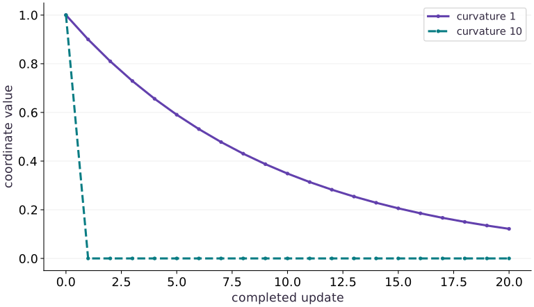
Predict before looking: At rate $0.1$ , which coordinate reaches zero immediately?

Read the figure

The horizontal axis counts completed updates; the point at $0$ is the initial state. The vertical axis shows a parameter coordinate, not the total loss. Both coordinates start at $1$ , but the coordinate with curvature $10$ drops to zero after one update, while the coordinate with curvature $1$ decays gradually.

The gradual curve starts $1,0.9,0.81$ and is still about $0.122$ after $20$ updates. The dashed curve remains at zero after its first drop. It has reached its optimum in this particular direction.

Connect it to the computation

For a quadratic direction with curvature $\lambda$ , gradient descent multiplies the coordinate by $1-\eta\lambda$ . At learning rate $0.1$ , that multiplier is $0.9$ for curvature $1$ and zero for curvature $10$ . The unequal curves come from curvature interacting with the same learning rate.

The steeper direction is faster here because the rate exactly cancels it. Increasing the rate further does not keep making it better: sufficiently large steps produce oscillation or divergence. This is why one shared rate can be constrained by a steep direction while making slow progress in a flatter one.

Open full-size figure Download data and provenance

The notebook contains the data experiment, plotting code, and recorded figure output. Rerun it to test your changes.

Where to put & run this code: Work in phases/04-optimization/08-curvature-hessians-and-learning-rates/code/main.py (or downloaded exercises/optimization-08.py / exercises/optimization-08.ipynb) and execute from the repository root with python3 phases/04-optimization/08-curvature-hessians-and-learning-rates/code/main.py.

1 Write the bowl

Create main.py with the objective and independently known curvature.

main.py · append build step 1

# Step 1 — Write the bowl: At the starting point the gradient is (1,10).
import jax
import jax.numpy as jnp

def loss(w):
    return 0.5 * (w[0] ** 2 + 10 * w[1] ** 2)
w = jnp.array([1.0, 1.0])
H = jnp.diag(jnp.array([1.0, 10.0]))
assert jnp.allclose(jax.grad(loss)(w), H @ w)

Code building blocks in this step

jnp.array(values, dtype=...) — Constructs an immutable device-backed JAX array from Python/NumPy values.
jnp.allclose(actual, expected, rtol=..., atol=...) — Checks that two arrays match elementwise within floating-point tolerance.
jax.grad(loss_fn)(params, ...) — Transforms a scalar-output function into a function returning the gradient PyTree with the same structure as params.

At the starting point the gradient is $(1,10)$ .

2 Check second derivatives

Append the full Hessian and a product check.

main.py · append build step 2

# Step 2 — Check second derivatives: The product agrees with the diagonal matrix without constructing a...
assert jnp.allclose(jax.hessian(loss)(w), H)
v = jnp.array([2.0, -1.0])
# Differentiate the objective to obtain `hv` via automatic differentiation.
hv = jax.jvp(jax.grad(loss), (w,), (v,))[1]
assert jnp.allclose(hv, jnp.array([2.0, -10.0]))

Code building blocks in this step

jnp.array(values, dtype=...) — Constructs an immutable device-backed JAX array from Python/NumPy values.
jnp.allclose(actual, expected, rtol=..., atol=...) — Checks that two arrays match elementwise within floating-point tolerance.
jax.grad(loss_fn)(params, ...) — Transforms a scalar-output function into a function returning the gradient PyTree with the same structure as params.
jax.jvp / jax.vjp / jax.jacfwd / jax.hessian — Computes exact forward-mode JVP, reverse-mode VJP, full Jacobians, or second-order curvature.

The product agrees with the diagonal matrix without constructing a Hessian inside the JVP.

3 Run an explicit trajectory

Append this scan and run python main.py. The history records losses after each update.

main.py · append build step 3

# Step 3 — Run an explicit trajectory: The second coordinate vanishes; the first remains near 0.1216...
# Define `run(rate, steps)` to evaluate the objective and its automatic derivatives:
def run(rate, steps=20):

    # Define `step(w, _)` to evaluate the objective and its automatic derivatives:
    def step(w, _):
        # Differentiate the objective to obtain `w` via automatic differentiation.
        w = w - rate * jax.grad(loss)(w)
        return (w, loss(w))
    return jax.lax.scan(step, jnp.array([1.0, 1.0]), None, length=steps)
final, history = run(0.1)
assert jnp.allclose(final, jnp.array([0.9 ** 20, 0.0]), atol=2e-06)
assert jnp.all(jnp.diff(history) <= 1e-06)
print('final weights / loss:', final, history[-1])

Code building blocks in this step

jnp.array(values, dtype=...) — Constructs an immutable device-backed JAX array from Python/NumPy values.
jnp.allclose(actual, expected, rtol=..., atol=...) — Checks that two arrays match elementwise within floating-point tolerance.
jax.grad(loss_fn)(params, ...) — Transforms a scalar-output function into a function returning the gradient PyTree with the same structure as params.
jax.lax.scan(step_fn, init_carry, xs, length=...) — Compiles a sequential loop where step_fn(carry, x) returns (next_carry, y), returning (final_carry, stacked_ys).

The second coordinate vanishes; the first remains near $0.1216$ after $20$ steps.

View the cumulative build in main.py

These blocks append in order to the same file.

main.py · cumulative Python build

# Step 1 — Write the bowl: At the starting point the gradient is (1,10).
import jax
import jax.numpy as jnp

def loss(w):
    return 0.5 * (w[0] ** 2 + 10 * w[1] ** 2)
w = jnp.array([1.0, 1.0])
H = jnp.diag(jnp.array([1.0, 10.0]))
assert jnp.allclose(jax.grad(loss)(w), H @ w)

# Step 2 — Check second derivatives: The product agrees with the diagonal matrix without constructing a...
assert jnp.allclose(jax.hessian(loss)(w), H)
v = jnp.array([2.0, -1.0])
# Differentiate the objective to obtain `hv` via automatic differentiation.
hv = jax.jvp(jax.grad(loss), (w,), (v,))[1]
assert jnp.allclose(hv, jnp.array([2.0, -10.0]))

# Step 3 — Run an explicit trajectory: The second coordinate vanishes; the first remains near 0.1216...
# Define `run(rate, steps)` to evaluate the objective and its automatic derivatives:
def run(rate, steps=20):

    # Define `step(w, _)` to evaluate the objective and its automatic derivatives:
    def step(w, _):
        # Differentiate the objective to obtain `w` via automatic differentiation.
        w = w - rate * jax.grad(loss)(w)
        return (w, loss(w))
    return jax.lax.scan(step, jnp.array([1.0, 1.0]), None, length=steps)
final, history = run(0.1)
assert jnp.allclose(final, jnp.array([0.9 ** 20, 0.0]), atol=2e-06)
assert jnp.all(jnp.diff(history) <= 1e-06)
print('final weights / loss:', final, history[-1])

Run the example

python3 phases/04-optimization/08-curvature-hessians-and-learning-rates/code/main.py

About this command

This shortcut uses an activated macOS/Linux course environment in the repository folder. For Windows, use the explicit interpreter command in “Setup help” above. The script includes worked examples and reference solutions.

Inspect the complete assembled example

main.py · complete Python example

# Step 1 — Write the bowl: At the starting point the gradient is (1,10).
import jax
import jax.numpy as jnp

def loss(w):
    return 0.5 * (w[0] ** 2 + 10 * w[1] ** 2)
w = jnp.array([1.0, 1.0])
H = jnp.diag(jnp.array([1.0, 10.0]))
assert jnp.allclose(jax.grad(loss)(w), H @ w)

# Step 2 — Check second derivatives: The product agrees with the diagonal matrix without constructing a...
assert jnp.allclose(jax.hessian(loss)(w), H)
v = jnp.array([2.0, -1.0])
# Differentiate the objective to obtain `hv` via automatic differentiation.
hv = jax.jvp(jax.grad(loss), (w,), (v,))[1]
assert jnp.allclose(hv, jnp.array([2.0, -10.0]))

# Step 3 — Run an explicit trajectory: The second coordinate vanishes; the first remains near 0.1216...
# Define `run(rate, steps)` to evaluate the objective and its automatic derivatives:
def run(rate, steps=20):

    # Define `step(w, _)` to evaluate the objective and its automatic derivatives:
    def step(w, _):
        # Differentiate the objective to obtain `w` via automatic differentiation.
        w = w - rate * jax.grad(loss)(w)
        return (w, loss(w))
    return jax.lax.scan(step, jnp.array([1.0, 1.0]), None, length=steps)
final, history = run(0.1)
assert jnp.allclose(final, jnp.array([0.9 ** 20, 0.0]), atol=2e-06)
assert jnp.all(jnp.diff(history) <= 1e-06)
print('final weights / loss:', final, history[-1])

Expected result: At rate $0.1$ , the final loss is about $0.00739$ and the trajectory is decreasing.

Recorded reference execution

Reference output captured from executing the complete lesson script (code/main.py) and its assertions in the course CPU environment.

2026-10-20T10:45:46.372064+00:00 · Python 3.14.3 · JAX 0.9.2 · 1 CPU device

final weights / loss: [ 0.12157664 -0.        ] 0.0073904395
final weights / loss: [ 0.12157664 -0.        ] 0.0073904395
PASS: optimization-08

Download execution record · The notebook includes executed cells and figure outputs. Compare your run with these values; timings depend on the machine.

Cross the stability boundary

Cross the stability boundary · Python experiment

# Experiment — Cross the stability boundary: A learning-rate bound depends on curvature, not on a universal...
edge, _ = run(0.2)
bad, bad_history = run(0.21)
assert jnp.allclose(jnp.abs(edge[1]), 1.0, atol=2e-06)
assert jnp.abs(bad[1]) > 6.0
assert bad_history[-1] > loss(w)

Expected: At the boundary its magnitude stays $1$ ; above it the magnitude grows.

A learning-rate bound depends on curvature, not on a universal default value.

Change coordinates

Change coordinates · Python experiment

# Experiment — Change coordinates: Coordinates can change optimization geometry while representing...
z = jnp.array([w[0], jnp.sqrt(10.0) * w[1]])
round_loss = lambda z: 0.5 * jnp.dot(z, z)
# Differentiate the objective to obtain `z_next` via automatic differentiation.
z_next = z - jax.grad(round_loss)(z)
assert jnp.allclose(z_next, jnp.zeros(2))
assert jnp.allclose(round_loss(z), loss(w))

Expected: The transformed objective starts at the same value and reaches zero in one step.

Coordinates can change optimization geometry while representing the same underlying objective.

Hands-On Exercise · Modify & Verify Run in the declared lesson environment

Make it yours

Where to put your code: Append your solution at the bottom of phases/04-optimization/08-curvature-hessians-and-learning-rates/code/main.py (or inside the Make it yours cell of exercises/optimization-08.ipynb) and run python3 phases/04-optimization/08-curvature-hessians-and-learning-rates/code/main.py to verify your prediction before opening the reference solution.

For curvatures $(2,8)$ , derive the stable interval and check one step at rate $0.1$ from $(1,1)$ .

Show a writing guide and starter scaffold

How to write this exercise code: step-by-step recipe & starter scaffold

1. Key functions & syntax to use:

jnp.array(values, dtype=...) — Constructs an immutable device-backed JAX array from Python/NumPy values.
jnp.allclose(actual, expected, rtol=..., atol=...) — Checks that two arrays match elementwise within floating-point tolerance.

2. Step-by-step implementation plan:

Set up the changed input or configuration parameters requested in the prompt.
Run the target function or transformation and assert that the output matches your prediction.

Starter code scaffold · copy into your file & fill in the TODOs

# Exercise solution: For curvatures (2,8), derive the stable interval and check one step at...
H2 = jnp.diag(...)  # TODO: compute H2
w_next = ...  # TODO: compute w_next
assert jnp.allclose(w_next, jnp.array([0.8, 0.2]), atol=1e-06)  # TODO: complete assertion check
assert jnp.allclose(2 / jnp.max(jnp.linalg.eigvalsh(H2)), 0.25)  # TODO: complete assertion check

Reveal the reference solution

Reference solution

# Exercise solution: For curvatures (2,8), derive the stable interval and check one step at...
H2 = jnp.diag(jnp.array([2.0, 8.0]))
w_next = w - 0.1 * (H2 @ w)
assert jnp.allclose(w_next, jnp.array([0.8, 0.2]), atol=1e-06)
assert jnp.allclose(2 / jnp.max(jnp.linalg.eigvalsh(H2)), 0.25)

Reject the zero-gradient shortcut

Transfer / diagnosis

At the origin of $S(w)=w_0^2-w_1^2$ , show zero gradient and both a lower and higher nearby value.

Show a writing guide and starter scaffold

How to write this practice solution: step-by-step recipe & starter scaffold

1. Key functions & syntax to use:

jnp.array(values, dtype=...) — Constructs an immutable device-backed JAX array from Python/NumPy values.
jnp.zeros / jnp.ones(shape, dtype=...) — Allocates a tensor of the given shape initialized with constants.
jnp.allclose(actual, expected, rtol=..., atol=...) — Checks that two arrays match elementwise within floating-point tolerance.
jax.grad(loss_fn)(params, ...) — Transforms a scalar-output function into a function returning the gradient PyTree with the same structure as params.

2. Step-by-step implementation plan:

Set up the changed input or configuration parameters requested in the prompt.
Run the target function or transformation and assert that the output matches your prediction.

Starter code scaffold · copy into your file & fill in the TODOs

# Reject the zero-gradient shortcut (Transfer / diagnosis): Stationarity is a first-order condition, not a proof of a...
saddle = ...  # TODO: compute saddle
zero = jnp.zeros(...)  # TODO: compute zero
assert jnp.allclose(jax.grad(saddle)(zero), zero)  # TODO: complete assertion check
assert saddle(jnp.array([0.0, 0.1]))  # TODO: complete assertion check
assert saddle(jnp.array([0.1, 0.0]))  # TODO: complete assertion check
assert jnp.allclose(jnp.linalg.eigvalsh(jax.hessian(saddle)(zero)), jnp.array([-2.0, 2.0]))  # TODO: complete assertion check

Show a hint

Move by $0.1$ along each axis separately.

Reveal reference solution and reasoning

Reject the zero-gradient shortcut · Python solution

# Reject the zero-gradient shortcut (Transfer / diagnosis): Stationarity is a first-order condition, not a proof of a...
saddle = lambda z: z[0] ** 2 - z[1] ** 2
zero = jnp.zeros(2)
assert jnp.allclose(jax.grad(saddle)(zero), zero)
assert saddle(jnp.array([0.0, 0.1])) < saddle(zero)
assert saddle(jnp.array([0.1, 0.0])) > saddle(zero)
assert jnp.allclose(jnp.linalg.eigvalsh(jax.hessian(saddle)(zero)), jnp.array([-2.0, 2.0]))

Stationarity is a first-order condition, not a proof of a minimum.

Transfer to a nonquadratic function

Transfer / diagnosis

For $F(w)=\sum_i e^{w_i}$ , verify a Hessian-vector product at $(0,\log 2)$ along $(1,3)$ .

Show a writing guide and starter scaffold

How to write this practice solution: step-by-step recipe & starter scaffold

1. Key functions & syntax to use:

jnp.array(values, dtype=...) — Constructs an immutable device-backed JAX array from Python/NumPy values.
x.sum(axis=...) / x.mean(axis=..., keepdims=...) — Reduces values along the named axis (the axis you name is collapsed unless keepdims=True).
jnp.allclose(actual, expected, rtol=..., atol=...) — Checks that two arrays match elementwise within floating-point tolerance.
jax.grad(loss_fn)(params, ...) — Transforms a scalar-output function into a function returning the gradient PyTree with the same structure as params.

2. Step-by-step implementation plan:

Differentiate the objective to obtain product via automatic differentiation.

Starter code scaffold · copy into your file & fill in the TODOs

# Transfer to a nonquadratic function (Transfer / diagnosis): For a nonquadratic function the Hessian changes with the...
point = jnp.array(...)  # TODO: compute point
direction = jnp.array(...)  # TODO: compute direction
# Differentiate the objective to obtain `product` via automatic differentiation.
product = jax.jvp(...)  # TODO: compute product
assert jnp.allclose(product, jnp.array([1.0, 6.0]), atol=1e-06)  # TODO: complete assertion check

Show a hint

The analytic Hessian is diagonal with entries $e^{w_i}$ .

Reveal reference solution and reasoning

Transfer to a nonquadratic function · Python solution

# Transfer to a nonquadratic function (Transfer / diagnosis): For a nonquadratic function the Hessian changes with the...
point = jnp.array([0.0, jnp.log(2.0)])
direction = jnp.array([1.0, 3.0])
# Differentiate the objective to obtain `product` via automatic differentiation.
product = jax.jvp(jax.grad(lambda z: jnp.sum(jnp.exp(z))), (point,), (direction,))[1]
assert jnp.allclose(product, jnp.array([1.0, 6.0]), atol=1e-06)

For a nonquadratic function the Hessian changes with the point; a bound from one location is not a global guarantee.

Diagnose the result

If a run oscillates or diverges, inspect the steepest curvature and the effective step size. If it barely moves, compare directional scales. If a zero gradient appears suspicious, probe nearby values before declaring success.

Carry forward

A learning-rate bound depends on curvature, not on a universal default value.
Coordinates can change optimization geometry while representing the same underlying objective.

Keep your evidence

Download evidence template

Keep the Hessian and Hessian-vector checks, stable/divergent trajectories, rescaling comparison and saddle counterexample.

Save your modified code, its output, and an explanation of your prediction. Checkpoint answers and exercise evidence are tracked separately.

Saved in this browser. Export or back up your portfolio anytime in My learning.

Save work for this lesson

Verified on local CPU. Stage to a Cloud TPU VM via Cloud TPU setup to record accelerator execution receipts (TODO: add automated Cloud TPU CI execution receipts).

Curvature, Hessians, and learning rates

What you will be able to do

The problem

The idea

Why one learning rate must respect the steep direction

Read a bowl through its curvature

Derive a stability bound

See why scaling helps

Distinguish a minimum from a stationary point

Unequal curvature produces unequal progress

Read the figure

Connect it to the computation

1 Write the bowl

2 Check second derivatives

3 Run an explicit trajectory

Run the example

Recorded reference execution

Cross the stability boundary

Change coordinates

Make it yours

Reject the zero-gradient shortcut

Transfer to a nonquadratic function

Check your understanding

Diagnose the result

Carry forward

Keep your evidence

Primary references