Core Foundation · Local CPULaptop CPULesson 4 of 12 in Phase 04

Phase 04 / Math & optimization

The chain rule, Jacobians, and directions

Revision v0.7.0 · 2026-10-20

Lesson · about 80 minutes · CPU practice

Compute a small Jacobian by hand and connect forward sensitivities to reverse-mode gradients.

Phase study guide: preparation, milestones and project evidence

Before you start

Before this: Least squares, rank, and conditioning
Hardware: CPU

Download notebook

Other downloads

Python worked examples Lesson text

Setup help: Python, notebook, or Cloud TPU VM

Use the tested CPU packages (the recorded environment uses Python 3.14.3). Other Python versions and accelerator environments require separate checks. The optional Cloud TPU specialization explains the target-specific execution boundaries. Logical CPU devices practice partitioning; they do not simulate TPU performance.

Download the repository ZIP or use your existing checkout. Extract it and open a terminal in the folder containing requirements-cpu.txt. The beginner ZIP is separate; these lessons use the full repository folder.

macOS / Linux terminal · repository folder

python3 -m venv .venv
source .venv/bin/activate
python -m pip install -r requirements-cpu.txt

PowerShell · repository folder

py -3 -m venv .venv
.\.venv\Scripts\python.exe -m pip install -r requirements-cpu.txt

After activation, run the complete worked example from that same folder:

macOS / Linux terminal · activated environment

python phases/04-optimization/07-chain-rule-jacobians-and-directional-derivatives/code/main.py

PowerShell command · repository folder

.\.venv\Scripts\python.exe phases/04-optimization/07-chain-rule-jacobians-and-directional-derivatives/code/main.py

For an incremental build, create main.py in your own practice folder, append each build block in order, and run python main.py with this environment active. Keep that file separate from the downloaded reference solution.

Download this lesson’s notebook. Open it with a Python kernel using the course environment. Run cells from the top after restarting the kernel; experiments depend on earlier definitions.

For local Jupyter, first install the course requirements using the Local Python steps, then use your environment’s Python to start Jupyter:

macOS / Linux terminal · activated course environment

python -m pip install jupyterlab
python -m jupyter lab

PowerShell command · repository folder

.\.venv\Scripts\python.exe -m pip install jupyterlab
.\.venv\Scripts\python.exe -m jupyter lab

Select the downloaded optimization-07.ipynb file in JupyterLab. The notebook contains reference solutions; make your prediction and attempt each practice task before opening them. Restart the kernel before changing logical device setup.

Check: Forward product $[3,1]$ , reverse product $[46,19]$ , directional loss derivative $27$ .

Revisit the guided CPU setup · Open 19: TPU Setup. Package instructions are CPU instructions; Windows and accelerator environments need their own validation.

Phase 04.04 Stage 1 of 5 · Understand

1 Understand 2 Build & Run 3 Experiment 4 Exercise & Check 5 Evidence

What you will be able to do

Compute a small Jacobian by hand and connect forward sensitivities to reverse-mode gradients.
Build a Jacobian one entry at a time
Push an input direction forward
Pull output sensitivity backward
Check both sides of the same calculation

The problem

One model input can affect several outputs. How does a small input change move those outputs, and how does a loss send sensitivity back? We will work through one tiny vector function before asking JAX to do the same calculation.

The idea

A Jacobian collects how each output responds to each input. We often need its action on a direction rather than the full matrix. Forward products move input perturbations to output perturbations; reverse products bring output sensitivities back to inputs.

Follow one direction through a Jacobian

Take $J=[[4,1],[3,2]]$ and input direction $v=[1,-1]$ . Multiplication gives $Jv=[3,1]$ . This predicts the first-order output change when we move a small distance along that direction.

For output sensitivity $u=[2,-1]$ , the reverse product is $J^Tu=[5,0]$ . These vectors live in different spaces even though both happen to have two entries in this example. Use unequal input/output dimensions in a follow-up test so equal lengths cannot hide a transpose mistake.

There is a useful independent agreement: $u^T(Jv)=5$ and $(J^Tu)^Tv=5$ . This checks the relationship between forward and reverse products without requiring you to inspect every Jacobian entry.

Build a Jacobian one entry at a time

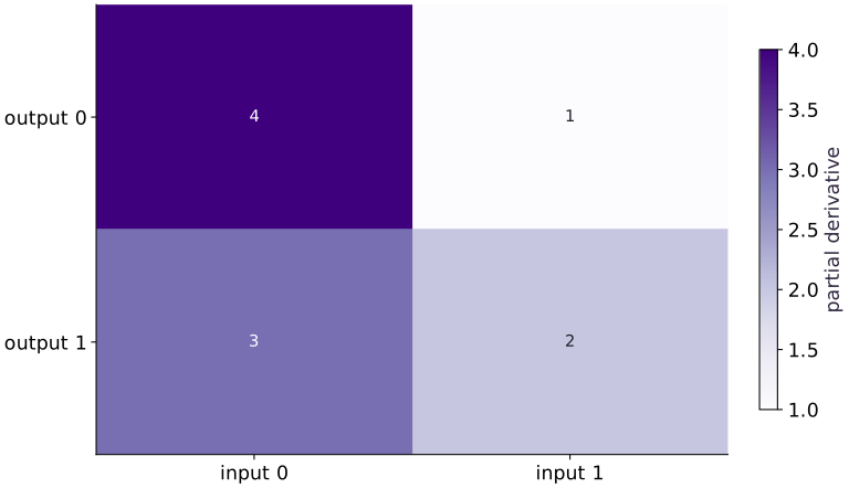
Let $f(x)=(x_0^2+x_1,\;x_0x_1)$ , where $x=(x_0,x_1)$ . The first output changes at rates $2x_0$ and $1$ ; the second changes at rates $x_1$ and $x_0$ . Rows describe outputs, columns describe inputs. At $x=(2,3)$ , the output is $(7,6)$ and the Jacobian is $J=\begin{pmatrix}4&1\\3&2\end{pmatrix}$ .

J_{ij}=\frac{\partial f_i}{\partial x_j},\qquad J\in\mathbb{R}^{m\times d}\ \text{for}\ f:\mathbb{R}^d\to\mathbb{R}^m

Push an input direction forward

Choose $v=(1,-1)$ . A small move $\varepsilon v$ in the input changes the output by approximately $\varepsilon Jv$ . Here $Jv=(3,1)$ : the first output moves three times as fast as the second along this direction. jax.jvp returns both the ordinary output and this directional sensitivity. It can compute the product without storing the full Jacobian.

f(x+\varepsilon v)\approx f(x)+\varepsilon Jv

Pull output sensitivity backward

Suppose the scalar loss is $L(x)=\tfrac12\|f(x)\|_2^2$ . Its derivative with respect to the outputs is $c=f(x)=(7,6)$ . The chain rule gives $\nabla_x L=J^\mathsf{T}c=(46,19)$ . jax.vjp returns the output and a pullback function. Passing $c$ into that function returns input sensitivities. The pullback result is a tuple because a function can have several inputs.

\nabla_x L=J^\mathsf{T}\nabla_f L

Check both sides of the same calculation

The identity $c^\mathsf{T}(Jv)=v^\mathsf{T}(J^\mathsf{T}c)$ checks that forward and reverse products agree. We also compare against the hand matrix and central differences so our evidence is not only two autodiff APIs agreeing. jax.grad needs a scalar output; use a Jacobian or a selected output direction for a vector function. These local derivatives do not describe a large move exactly.

A Jacobian maps inputs to output sensitivities

Predict before looking: Which output is more sensitive to the first input at $(2,3)$ ?

Read the figure

Rows identify output coordinates and columns identify input coordinates. Each cell is a partial derivative evaluated at the example input $(2,3)$ . The matrix is $J=\begin{pmatrix}4&1\\3&2\end{pmatrix}$ , and darker cells indicate larger positive sensitivity here.

Read down the first column: a small increase in input $0$ , holding input $1$ fixed, changes the two outputs by approximately $4$ and $3$ times that increase. Read across the first row to see how both inputs influence output $0$ .

Connect it to the computation

For a joint input change in direction $v=(1,-1)$ , multiply the whole matrix by that direction: $Jv=(3,1)$ . The second input’s decrease offsets some of the first input’s increase. Looking only at the darkest cell would miss that interaction.

These are local sensitivities, not model weights, probabilities, or final output values. The entries can change at another input. To check the interpretation, take a small step $\epsilon v$ and compare the output change with $\epsilon Jv$ .

Open full-size figure Download data and provenance

The notebook contains the data experiment, plotting code, and recorded figure output. Rerun it to test your changes.

Where to put & run this code: Work in phases/04-optimization/07-chain-rule-jacobians-and-directional-derivatives/code/main.py (or downloaded exercises/optimization-07.py / exercises/optimization-07.ipynb) and execute from the repository root with python3 phases/04-optimization/07-chain-rule-jacobians-and-directional-derivatives/code/main.py.

1 Write the vector function

Create main.py. Define the function, its input and the hand-derived Jacobian.

main.py · append build step 1

# Step 1 — Write the vector function: The matrix is written from the derivatives, not obtained from an...
import jax
import jax.numpy as jnp

def f(x):
    return jnp.array([x[0] ** 2 + x[1], x[0] * x[1]])
x = jnp.array([2.0, 3.0])
v = jnp.array([1.0, -1.0])
J = jnp.array([[4.0, 1.0], [3.0, 2.0]])
assert jnp.allclose(f(x), jnp.array([7.0, 6.0]))

Code building blocks in this step

jnp.array(values, dtype=...) — Constructs an immutable device-backed JAX array from Python/NumPy values.
jnp.allclose(actual, expected, rtol=..., atol=...) — Checks that two arrays match elementwise within floating-point tolerance.

The matrix is written from the derivatives, not obtained from an autodiff call.

2 Push a direction and pull a sensitivity

Append these two transformations; predict both products first.

main.py · append build step 2

# Step 2 — Push a direction and pull a sensitivity: Forward mode follows an input direction; reverse mode starts with...
# Compute exact directional derivative / Jacobian / Hessian (`(out, jv)`).
out, jv = jax.jvp(f, (x,), (v,))
# Compute exact directional derivative / Jacobian / Hessian (`(_, pullback)`).
_, pullback = jax.vjp(f, x)
c = out
jt_c = pullback(c)[0]
assert jnp.allclose(jv, jnp.array([3.0, 1.0]))
assert jnp.allclose(jt_c, jnp.array([46.0, 19.0]))

Code building blocks in this step

jnp.array(values, dtype=...) — Constructs an immutable device-backed JAX array from Python/NumPy values.
jnp.allclose(actual, expected, rtol=..., atol=...) — Checks that two arrays match elementwise within floating-point tolerance.
jax.jvp / jax.vjp / jax.jacfwd / jax.hessian — Computes exact forward-mode JVP, reverse-mode VJP, full Jacobians, or second-order curvature.

Forward mode follows an input direction; reverse mode starts with output sensitivity.

3 Connect to a scalar loss

Append the scalar objective and independent matrix checks, then run python main.py.

main.py · append build step 3

# Step 3 — Connect to a scalar loss: Both routes give directional loss derivative 27.
def loss(x):
    return 0.5 * jnp.sum(f(x) ** 2)
assert jnp.allclose(jax.jacfwd(f)(x), J)
assert jnp.allclose(jax.grad(loss)(x), J.T @ c)
assert jnp.allclose(jnp.dot(c, jv), jnp.dot(v, jt_c))
print('Jv / loss gradient:', jv, jt_c)

Code building blocks in this step

x.sum(axis=...) / x.mean(axis=..., keepdims=...) — Reduces values along the named axis (the axis you name is collapsed unless keepdims=True).
jnp.allclose(actual, expected, rtol=..., atol=...) — Checks that two arrays match elementwise within floating-point tolerance.
jax.grad(loss_fn)(params, ...) — Transforms a scalar-output function into a function returning the gradient PyTree with the same structure as params.
jax.jvp / jax.vjp / jax.jacfwd / jax.hessian — Computes exact forward-mode JVP, reverse-mode VJP, full Jacobians, or second-order curvature.

Both routes give directional loss derivative $27$ .

View the cumulative build in main.py

These blocks append in order to the same file.

main.py · cumulative Python build

# Step 1 — Write the vector function: The matrix is written from the derivatives, not obtained from an...
import jax
import jax.numpy as jnp

def f(x):
    return jnp.array([x[0] ** 2 + x[1], x[0] * x[1]])
x = jnp.array([2.0, 3.0])
v = jnp.array([1.0, -1.0])
J = jnp.array([[4.0, 1.0], [3.0, 2.0]])
assert jnp.allclose(f(x), jnp.array([7.0, 6.0]))

# Step 2 — Push a direction and pull a sensitivity: Forward mode follows an input direction; reverse mode starts with...
# Compute exact directional derivative / Jacobian / Hessian (`(out, jv)`).
out, jv = jax.jvp(f, (x,), (v,))
# Compute exact directional derivative / Jacobian / Hessian (`(_, pullback)`).
_, pullback = jax.vjp(f, x)
c = out
jt_c = pullback(c)[0]
assert jnp.allclose(jv, jnp.array([3.0, 1.0]))
assert jnp.allclose(jt_c, jnp.array([46.0, 19.0]))

# Step 3 — Connect to a scalar loss: Both routes give directional loss derivative 27.
def loss(x):
    return 0.5 * jnp.sum(f(x) ** 2)
assert jnp.allclose(jax.jacfwd(f)(x), J)
assert jnp.allclose(jax.grad(loss)(x), J.T @ c)
assert jnp.allclose(jnp.dot(c, jv), jnp.dot(v, jt_c))
print('Jv / loss gradient:', jv, jt_c)

Run the example

python3 phases/04-optimization/07-chain-rule-jacobians-and-directional-derivatives/code/main.py

About this command

This shortcut uses an activated macOS/Linux course environment in the repository folder. For Windows, use the explicit interpreter command in “Setup help” above. The script includes worked examples and reference solutions.

Inspect the complete assembled example

main.py · complete Python example

# Step 1 — Write the vector function: The matrix is written from the derivatives, not obtained from an...
import jax
import jax.numpy as jnp

def f(x):
    return jnp.array([x[0] ** 2 + x[1], x[0] * x[1]])
x = jnp.array([2.0, 3.0])
v = jnp.array([1.0, -1.0])
J = jnp.array([[4.0, 1.0], [3.0, 2.0]])
assert jnp.allclose(f(x), jnp.array([7.0, 6.0]))

# Step 2 — Push a direction and pull a sensitivity: Forward mode follows an input direction; reverse mode starts with...
# Compute exact directional derivative / Jacobian / Hessian (`(out, jv)`).
out, jv = jax.jvp(f, (x,), (v,))
# Compute exact directional derivative / Jacobian / Hessian (`(_, pullback)`).
_, pullback = jax.vjp(f, x)
c = out
jt_c = pullback(c)[0]
assert jnp.allclose(jv, jnp.array([3.0, 1.0]))
assert jnp.allclose(jt_c, jnp.array([46.0, 19.0]))

# Step 3 — Connect to a scalar loss: Both routes give directional loss derivative 27.
def loss(x):
    return 0.5 * jnp.sum(f(x) ** 2)
assert jnp.allclose(jax.jacfwd(f)(x), J)
assert jnp.allclose(jax.grad(loss)(x), J.T @ c)
assert jnp.allclose(jnp.dot(c, jv), jnp.dot(v, jt_c))
print('Jv / loss gradient:', jv, jt_c)

Expected result: Forward product $[3,1]$ , reverse product $[46,19]$ , directional loss derivative $27$ .

Recorded reference execution

Reference output captured from executing the complete lesson script (code/main.py) and its assertions in the course CPU environment.

2026-10-20T10:45:39.979446+00:00 · Python 3.14.3 · JAX 0.9.2 · 1 CPU device

Jv / loss gradient: [3. 1.] [46. 19.]
Jv / loss gradient: [3. 1.] [46. 19.]
PASS: optimization-07

Download execution record · The notebook includes executed cells and figure outputs. Compare your run with these values; timings depend on the machine.

Check a finite input move

Check a finite input move · Python experiment

# Experiment — Check a finite input move: A numerical perturbation provides a check independent of autodiff.
h = 0.01
fd = (f(x + h * v) - f(x - h * v)) / (2 * h)
assert jnp.allclose(fd, J @ v, atol=0.0001, rtol=0.0001)

Expected: The finite-direction and hand-matrix results agree within float32 tolerance.

A numerical perturbation provides a check independent of autodiff.

Change the point

Change the point · Python experiment

# Experiment — Change the point: The Jacobian describes sensitivity at the current point; it is...
x2 = jnp.array([0.0, 1.0])
J2 = jnp.array([[0.0, 1.0], [1.0, 0.0]])
assert jnp.allclose(jax.jacrev(f)(x2), J2)
assert jnp.allclose(jax.jvp(f, (x2,), (v,))[1], J2 @ v)

Expected: The new Jacobian swaps the direction coordinates.

The Jacobian describes sensitivity at the current point; it is not generally constant.

Hands-On Exercise · Modify & Verify Run in the declared lesson environment

Make it yours

Where to put your code: Append your solution at the bottom of phases/04-optimization/07-chain-rule-jacobians-and-directional-derivatives/code/main.py (or inside the Make it yours cell of exercises/optimization-07.ipynb) and run python3 phases/04-optimization/07-chain-rule-jacobians-and-directional-derivatives/code/main.py to verify your prediction before opening the reference solution.

Replace the scalar loss by $L(x)=f_0(x)+2f_1(x)$ . Predict its gradient at $(2,3)$ before using grad.

Show a writing guide and starter scaffold

How to write this exercise code: step-by-step recipe & starter scaffold

1. Key functions & syntax to use:

jnp.array(values, dtype=...) — Constructs an immutable device-backed JAX array from Python/NumPy values.
jnp.allclose(actual, expected, rtol=..., atol=...) — Checks that two arrays match elementwise within floating-point tolerance.
jax.grad(loss_fn)(params, ...) — Transforms a scalar-output function into a function returning the gradient PyTree with the same structure as params.

2. Step-by-step implementation plan:

Set up the changed input or configuration parameters requested in the prompt.
Run the target function or transformation and assert that the output matches your prediction.

Starter code scaffold · copy into your file & fill in the TODOs

# Exercise solution: Replace the scalar loss by L(x)=f_0(x)+2f_1(x).
def weighted_loss(x):
    return ...  # TODO: return computed result
assert jnp.allclose(jax.grad(weighted_loss)(x), jnp.array([10.0, 5.0]))  # TODO: complete assertion check

Reveal the reference solution

Reference solution

# Exercise solution: Replace the scalar loss by L(x)=f_0(x)+2f_1(x).
def weighted_loss(x):
    return f(x)[0] + 2 * f(x)[1]
assert jnp.allclose(jax.grad(weighted_loss)(x), jnp.array([10.0, 5.0]))

Find the broken derivative path

Transfer / diagnosis

A colleague wraps the first input in jax.lax.stop_gradient. The forward outputs are unchanged. Show why the gradient no longer matches the intended mathematical function.

Show a writing guide and starter scaffold

How to write this practice solution: step-by-step recipe & starter scaffold

1. Key functions & syntax to use:

jnp.array(values, dtype=...) — Constructs an immutable device-backed JAX array from Python/NumPy values.
x.sum(axis=...) / x.mean(axis=..., keepdims=...) — Reduces values along the named axis (the axis you name is collapsed unless keepdims=True).
jnp.allclose(actual, expected, rtol=..., atol=...) — Checks that two arrays match elementwise within floating-point tolerance.
jax.grad(loss_fn)(params, ...) — Transforms a scalar-output function into a function returning the gradient PyTree with the same structure as params.

2. Step-by-step implementation plan:

Define detached(x) to evaluate the objective and its automatic derivatives:

Starter code scaffold · copy into your file & fill in the TODOs

# Find the broken derivative path (Transfer / diagnosis): Equal forward values do not imply equal differentiation...
# Define `detached(x)` to evaluate the objective and its automatic derivatives:
def detached(x):
    a = jax.lax.stop_gradient(...)  # TODO: compute a
    return ...  # TODO: return computed result
assert jnp.allclose(detached(x), f(x))  # TODO: complete assertion check
assert jnp.allclose(jax.grad(lambda z: jnp.sum(detached(z)))(x), jnp.array([0.0, 3.0]))  # TODO: complete assertion check
assert jnp.allclose(jax.grad(lambda z: jnp.sum(f(z)))(x), jnp.array([7.0, 3.0]))  # TODO: complete assertion check

Show a hint

Compare the derivative of the sum of outputs with $J^\mathsf{T}(1,1)$ .

Reveal reference solution and reasoning

Find the broken derivative path · Python solution

# Find the broken derivative path (Transfer / diagnosis): Equal forward values do not imply equal differentiation...
# Define `detached(x)` to evaluate the objective and its automatic derivatives:
def detached(x):
    a = jax.lax.stop_gradient(x[0])
    return jnp.array([a * a + x[1], a * x[1]])
assert jnp.allclose(detached(x), f(x))
assert jnp.allclose(jax.grad(lambda z: jnp.sum(detached(z)))(x), jnp.array([0.0, 3.0]))
assert jnp.allclose(jax.grad(lambda z: jnp.sum(f(z)))(x), jnp.array([7.0, 3.0]))

Equal forward values do not imply equal differentiation behavior when derivative rules are deliberately changed.

Transfer to unequal dimensions

Transfer / diagnosis

For a matrix $A\in\mathbb{R}^{3\times2}$ , check that the VJP of $Ax$ maps an output sensitivity of length $3$ into a vector of length $2$ .

Show a writing guide and starter scaffold

How to write this practice solution: step-by-step recipe & starter scaffold

1. Key functions & syntax to use:

jnp.array(values, dtype=...) — Constructs an immutable device-backed JAX array from Python/NumPy values.
jnp.allclose(actual, expected, rtol=..., atol=...) — Checks that two arrays match elementwise within floating-point tolerance.
jax.jvp / jax.vjp / jax.jacfwd / jax.hessian — Computes exact forward-mode JVP, reverse-mode VJP, full Jacobians, or second-order curvature.

2. Step-by-step implementation plan:

Compute exact directional derivative / Jacobian / Hessian ((_, back)).
Check tensor shape invariant: back(c3)[0].shape == (2,)

Starter code scaffold · copy into your file & fill in the TODOs

# Transfer to unequal dimensions (Transfer / diagnosis): Unequal input and output dimensions make a mistaken...
A = jnp.array(...)  # TODO: compute A
c3 = jnp.array(...)  # TODO: compute c3
# Compute exact directional derivative / Jacobian / Hessian (`(_, back)`).
_, back = jax.vjp(...)  # TODO: compute _, back
# Check tensor shape invariant: `back(c3)[0].shape == (2,)`
assert back(c3)[0].shape  # TODO: complete assertion check
assert jnp.allclose(back(c3)[0], jnp.array([3.0, 0.0]))  # TODO: complete assertion check

Show a hint

The reference is $A^\mathsf{T}c$ , not $Ac$ .

Reveal reference solution and reasoning

Transfer to unequal dimensions · Python solution

# Transfer to unequal dimensions (Transfer / diagnosis): Unequal input and output dimensions make a mistaken...
A = jnp.array([[1.0, 0.0], [0.0, 2.0], [1.0, 1.0]])
c3 = jnp.array([1.0, -1.0, 2.0])
# Compute exact directional derivative / Jacobian / Hessian (`(_, back)`).
_, back = jax.vjp(lambda z: A @ z, x)
# Check tensor shape invariant: `back(c3)[0].shape == (2,)`
assert back(c3)[0].shape == (2,)
assert jnp.allclose(back(c3)[0], jnp.array([3.0, 0.0]))

Unequal input and output dimensions make a mistaken transpose visible.

Diagnose the result

If shapes fail, write output-by-input Jacobian dimensions on paper. If values match but derivatives do not, inspect stop_gradient, indexing, nondifferentiable operations and the scalar loss definition.

Carry forward

A numerical perturbation provides a check independent of autodiff.
The Jacobian describes sensitivity at the current point; it is not generally constant.

Keep your evidence

Download evidence template

Keep the handwritten Jacobian, JVP and VJP checks, adjoint identity, finite-direction check and stop-gradient diagnosis.

Save your modified code, its output, and an explanation of your prediction. Checkpoint answers and exercise evidence are tracked separately.

Saved in this browser. Export or back up your portfolio anytime in My learning.

Save work for this lesson

Verified on local CPU. Stage to a Cloud TPU VM via Cloud TPU setup to record accelerator execution receipts (TODO: add automated Cloud TPU CI execution receipts).

Primary references

JAX autodiff cookbook: JVPs and VJPs ↗

The chain rule, Jacobians, and directions

What you will be able to do

The problem

The idea

Follow one direction through a Jacobian

Build a Jacobian one entry at a time

Push an input direction forward

Pull output sensitivity backward

Check both sides of the same calculation

A Jacobian maps inputs to output sensitivities

Read the figure

Connect it to the computation

1 Write the vector function

2 Push a direction and pull a sensitivity

3 Connect to a scalar loss

Run the example

Recorded reference execution

Check a finite input move

Change the point

Make it yours

Find the broken derivative path

Transfer to unequal dimensions

Check your understanding

Diagnose the result

Carry forward

Keep your evidence

Primary references