Core Foundation · Local CPULaptop CPULesson 8 of 12 in Phase 04

Phase 04 / Math & optimization

Probability, likelihood, and stable losses

Revision v0.7.0 · 2026-10-20

Lesson · about 80 minutes · CPU practice

Derive binary cross-entropy from a probability model and compute it safely from logits.

Phase study guide: preparation, milestones and project evidence

Before you start

Before this: Write gradient descent yourself
Hardware: CPU

Download notebook

Other downloads

Python worked examples Lesson text

Setup help: Python, notebook, or Cloud TPU VM

Use the tested CPU packages (the recorded environment uses Python 3.14.3). Other Python versions and accelerator environments require separate checks. The optional Cloud TPU specialization explains the target-specific execution boundaries. Logical CPU devices practice partitioning; they do not simulate TPU performance.

Download the repository ZIP or use your existing checkout. Extract it and open a terminal in the folder containing requirements-cpu.txt. The beginner ZIP is separate; these lessons use the full repository folder.

macOS / Linux terminal · repository folder

python3 -m venv .venv
source .venv/bin/activate
python -m pip install -r requirements-cpu.txt

PowerShell · repository folder

py -3 -m venv .venv
.\.venv\Scripts\python.exe -m pip install -r requirements-cpu.txt

After activation, run the complete worked example from that same folder:

macOS / Linux terminal · activated environment

python phases/04-optimization/09-probability-likelihood-and-stable-losses/code/main.py

PowerShell command · repository folder

.\.venv\Scripts\python.exe phases/04-optimization/09-probability-likelihood-and-stable-losses/code/main.py

For an incremental build, create main.py in your own practice folder, append each build block in order, and run python main.py with this environment active. Keep that file separate from the downloaded reference solution.

Download this lesson’s notebook. Open it with a Python kernel using the course environment. Run cells from the top after restarting the kernel; experiments depend on earlier definitions.

For local Jupyter, first install the course requirements using the Local Python steps, then use your environment’s Python to start Jupyter:

macOS / Linux terminal · activated course environment

python -m pip install jupyterlab
python -m jupyter lab

PowerShell command · repository folder

.\.venv\Scripts\python.exe -m pip install jupyterlab
.\.venv\Scripts\python.exe -m jupyter lab

Select the downloaded optimization-09.ipynb file in JupyterLab. The notebook contains reference solutions; make your prediction and attempt each practice task before opening them. Restart the kernel before changing logical device setup.

Check: Uncertain loss about $0.6931$ ; confident-wrong loss $100$ .

Revisit the guided CPU setup · Open 19: TPU Setup. Package instructions are CPU instructions; Windows and accelerator environments need their own validation.

Phase 04.08 Stage 1 of 5 · Understand

1 Understand 2 Build & Run 3 Experiment 4 Exercise & Check 5 Evidence

What you will be able to do

Derive binary cross-entropy from a probability model and compute it safely from logits.
Read likelihood as support for the observed data
Move from probabilities to logits
Avoid overflowing intermediate values
Extend the idea without overstating it

The problem

A classifier should tell us how strongly it believes a label, not only which label it chooses. How do we turn that belief into a loss? We will start with a yes-or-no event, derive the penalty for a prediction, and discover why an algebraically correct formula can fail on a computer.

The idea

A classification loss rewards probability assigned to the observed outcome. A logit is an unconstrained score that becomes a probability through a link such as the sigmoid. Stable formulas let us compute the same objective without overflowing or taking the logarithm of a rounded zero.

Connect a logit to the observed label

For a binary label of one, predicting probability $0.5$ gives loss $-\log(0.5)\approx0.693$ . Predicting $0.9$ gives about $0.105$ . If the observed label is instead zero, that same $0.9$ prediction gives $-\log(0.1)\approx2.303$ . Confidence helps only when it supports the observed outcome.

At logit zero, the sigmoid gives $0.5$ , so either binary label has the same loss. Moving the logit right helps the positive label and hurts the negative one. Follow the correct label's curve rather than treating a lower curve as universally better.

Extreme logits expose numerical differences between mathematically equivalent formulas. Prefer a stable logit-based loss and verify it against moderate-value hand calculations before exploring extreme cases.

Read likelihood as support for the observed data

The Bernoulli model writes the probability of an observed label as $p^y(1-p)^{1-y}$ . If the label is $1$ , predictions $p=0.8$ and $p=0.2$ incur losses about $0.2231$ and $1.6094$ , respectively. Both can be compared even before applying a classification threshold. For independent observations conditional on their inputs and model parameters, likelihoods multiply. Taking negative logarithms turns the product into a sum; dividing by the sample count gives a mean.

\ell(p,y)=-y\log p-(1-y)\log(1-p)

Move from probabilities to logits

A logit $z$ is an unrestricted real score. The sigmoid maps it into a probability: $p=1/(1+e^{-z})$ . At $z=0$ , the probability is $1/2$ and either binary label has loss $\log 2$ . For a positive label, differentiating the loss gives $p-1$ , so gradient descent increases the logit. More generally the derivative is $p-y$ . A very wrong, confident prediction still supplies a useful gradient.

\ell(z,y)=\operatorname{softplus}(z)-yz,\qquad \frac{\partial\ell}{\partial z}=\operatorname{sigmoid}(z)-y

Avoid overflowing intermediate values

Computing log(sigmoid(z)) directly can take a logarithm of a rounded zero. For $z=-100$ and $y=1$ , the correct loss is close to $100$ , not infinity. Use jax.nn.softplus or an established logits-based loss. The equivalent expression below explains the stability: its exponential argument is never positive. We use the library softplus for differentiation rather than hand-assembling maximum and abs, whose derivative conventions at a tie need care.

\operatorname{softplus}(z)=\max(z,0)+\log(1+e^{-|z|})

Extend the idea without overstating it

For mutually exclusive classes, the probability of class $k$ is the softmax of its score $z_k$ . Use jax.nn.log_softmax and select the observed class. Adding the same constant to every score must not change the probabilities or loss. A low training cross-entropy is not proof of calibration or generalization; check held-out predictions. Squared error also has a likelihood interpretation under independent Gaussian errors with fixed variance, but that assumption differs from the Bernoulli model.

\ell(z,y)=\log\!\left(\sum_k e^{z_k}\right)-z_y

Confidence is rewarded only when it matches the label

Predict before looking: For a positive label, which direction should the logit move?

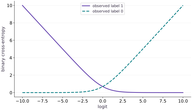
$Confidence is rewarded only when it matches the label. The horizontal axis is a logit, which becomes the predicted probability of label $1$ after a sigmoid. The vertical axis is binary cross-entropy loss. The solid curve assumes the observed label is $1$; the dashed curve assumes it is $0$. At logit $0$, the predicted probability is $0.5$, and both losses are $\log 2\approx0.693$. Moving right lowers the loss for observed label $1$ but raises it for observed label $0$. At logit $10$, the latter loss is about $10$, while the former is close to zero.$

Plot from a recorded CPU computation · JAX 0.9.2 · 1 CPU device

Read the figure

The horizontal axis is a logit, which becomes the predicted probability of label $1$ after a sigmoid. The vertical axis is binary cross-entropy loss. The solid curve assumes the observed label is $1$ ; the dashed curve assumes it is $0$ .

At logit $0$ , the predicted probability is $0.5$ , and both losses are $\log 2\approx0.693$ . Moving right lowers the loss for observed label $1$ but raises it for observed label $0$ . At logit $10$ , the latter loss is about $10$ , while the former is close to zero.

Connect it to the computation

A large positive logit strongly favors label $1$ . That confidence is rewarded only if label $1$ is actually observed. For label $0$ , the same confidence is a large mistake. The mirror-image curves make the dependence on the target explicit.

Loss is not a probability or classification accuracy, so values above $1$ are valid. The near-flat parts approach zero without implying an exact zero probability for the other class. Computing this loss from logits with a stable formula avoids unnecessary overflow or taking the logarithm of a rounded zero.

Open full-size figure Download data and provenance

The notebook contains the data experiment, plotting code, and recorded figure output. Rerun it to test your changes.

Where to put & run this code: Work in phases/04-optimization/09-probability-likelihood-and-stable-losses/code/main.py (or downloaded exercises/optimization-09.py / exercises/optimization-09.ipynb) and execute from the repository root with python3 phases/04-optimization/09-probability-likelihood-and-stable-losses/code/main.py.

1 Write a loss from logits

Create main.py. Start at an uncertain prediction so you can verify the answer by hand.

main.py · append build step 1

# Step 1 — Write a loss from logits: A balanced probability assigns loss \log 2 to either outcome.
import jax
import jax.numpy as jnp
import optax

def binary_loss(z, y):
    return jax.nn.softplus(z) - y * z
z = jnp.array(0.0)
y = jnp.array(1.0)
assert jnp.allclose(binary_loss(z, y), jnp.log(2.0))

Code building blocks in this step

jnp.array(values, dtype=...) — Constructs an immutable device-backed JAX array from Python/NumPy values.
jnp.allclose(actual, expected, rtol=..., atol=...) — Checks that two arrays match elementwise within floating-point tolerance.

A balanced probability assigns loss $\log 2$ to either outcome.

2 Check the derivative independently

Append the analytic gradient and a library comparison at moderate scores.

main.py · append build step 2

# Step 2 — Check the derivative independently: The derivative points toward assigning more probability to the...
assert jnp.allclose(jax.grad(binary_loss)(z, y), -0.5)
logits = jnp.array([-2.0, 0.0, 2.0])
labels = jnp.array([0.0, 1.0, 1.0])
analytic = jax.nn.sigmoid(logits) - labels
# Differentiate the objective to obtain `actual` via automatic differentiation.
actual = jax.vmap(jax.grad(binary_loss))(logits, labels)
assert jnp.allclose(actual, analytic, atol=1e-06)
assert jnp.allclose(binary_loss(logits, labels), optax.sigmoid_binary_cross_entropy(logits, labels), atol=1e-06)

Code building blocks in this step

jnp.array(values, dtype=...) — Constructs an immutable device-backed JAX array from Python/NumPy values.
jnp.allclose(actual, expected, rtol=..., atol=...) — Checks that two arrays match elementwise within floating-point tolerance.
jax.grad(loss_fn)(params, ...) — Transforms a scalar-output function into a function returning the gradient PyTree with the same structure as params.
jax.vmap(fn, in_axes=..., out_axes=...) — Vectorizes a single-example function across a batch axis without writing a Python loop.

The derivative points toward assigning more probability to the observed label.

3 Check a confident mistake

Append the extreme case and run python main.py.

main.py · append build step 3

# Step 3 — Check a confident mistake: The confident mistake has a large finite loss and derivative near -1.
assert jnp.allclose(binary_loss(jnp.array(-100.0), jnp.array(1.0)), 100.0)
assert jnp.allclose(jax.grad(binary_loss)(jnp.array(-100.0), jnp.array(1.0)), -1.0)
print('uncertain loss / confident-wrong loss:', binary_loss(z, y), binary_loss(-100.0, 1.0))

Code building blocks in this step

jnp.array(values, dtype=...) — Constructs an immutable device-backed JAX array from Python/NumPy values.
jnp.allclose(actual, expected, rtol=..., atol=...) — Checks that two arrays match elementwise within floating-point tolerance.
jax.grad(loss_fn)(params, ...) — Transforms a scalar-output function into a function returning the gradient PyTree with the same structure as params.

The confident mistake has a large finite loss and derivative near $-1$ .

View the cumulative build in main.py

These blocks append in order to the same file.

main.py · cumulative Python build

# Step 1 — Write a loss from logits: A balanced probability assigns loss \log 2 to either outcome.
import jax
import jax.numpy as jnp
import optax

def binary_loss(z, y):
    return jax.nn.softplus(z) - y * z
z = jnp.array(0.0)
y = jnp.array(1.0)
assert jnp.allclose(binary_loss(z, y), jnp.log(2.0))

# Step 2 — Check the derivative independently: The derivative points toward assigning more probability to the...
assert jnp.allclose(jax.grad(binary_loss)(z, y), -0.5)
logits = jnp.array([-2.0, 0.0, 2.0])
labels = jnp.array([0.0, 1.0, 1.0])
analytic = jax.nn.sigmoid(logits) - labels
# Differentiate the objective to obtain `actual` via automatic differentiation.
actual = jax.vmap(jax.grad(binary_loss))(logits, labels)
assert jnp.allclose(actual, analytic, atol=1e-06)
assert jnp.allclose(binary_loss(logits, labels), optax.sigmoid_binary_cross_entropy(logits, labels), atol=1e-06)

# Step 3 — Check a confident mistake: The confident mistake has a large finite loss and derivative near -1.
assert jnp.allclose(binary_loss(jnp.array(-100.0), jnp.array(1.0)), 100.0)
assert jnp.allclose(jax.grad(binary_loss)(jnp.array(-100.0), jnp.array(1.0)), -1.0)
print('uncertain loss / confident-wrong loss:', binary_loss(z, y), binary_loss(-100.0, 1.0))

Run the example

python3 phases/04-optimization/09-probability-likelihood-and-stable-losses/code/main.py

About this command

This shortcut uses an activated macOS/Linux course environment in the repository folder. For Windows, use the explicit interpreter command in “Setup help” above. The script includes worked examples and reference solutions.

Inspect the complete assembled example

main.py · complete Python example

# Step 1 — Write a loss from logits: A balanced probability assigns loss \log 2 to either outcome.
import jax
import jax.numpy as jnp
import optax

def binary_loss(z, y):
    return jax.nn.softplus(z) - y * z
z = jnp.array(0.0)
y = jnp.array(1.0)
assert jnp.allclose(binary_loss(z, y), jnp.log(2.0))

# Step 2 — Check the derivative independently: The derivative points toward assigning more probability to the...
assert jnp.allclose(jax.grad(binary_loss)(z, y), -0.5)
logits = jnp.array([-2.0, 0.0, 2.0])
labels = jnp.array([0.0, 1.0, 1.0])
analytic = jax.nn.sigmoid(logits) - labels
# Differentiate the objective to obtain `actual` via automatic differentiation.
actual = jax.vmap(jax.grad(binary_loss))(logits, labels)
assert jnp.allclose(actual, analytic, atol=1e-06)
assert jnp.allclose(binary_loss(logits, labels), optax.sigmoid_binary_cross_entropy(logits, labels), atol=1e-06)

# Step 3 — Check a confident mistake: The confident mistake has a large finite loss and derivative near -1.
assert jnp.allclose(binary_loss(jnp.array(-100.0), jnp.array(1.0)), 100.0)
assert jnp.allclose(jax.grad(binary_loss)(jnp.array(-100.0), jnp.array(1.0)), -1.0)
print('uncertain loss / confident-wrong loss:', binary_loss(z, y), binary_loss(-100.0, 1.0))

Expected result: Uncertain loss about $0.6931$ ; confident-wrong loss $100$ .

Recorded reference execution

Reference output captured from executing the complete lesson script (code/main.py) and its assertions in the course CPU environment.

2026-10-20T10:45:52.039722+00:00 · Python 3.14.3 · JAX 0.9.2 · 1 CPU device

uncertain loss / confident-wrong loss: 0.6931472 100.0
uncertain loss / confident-wrong loss: 0.6931472 100.0
PASS: optimization-09

Download execution record · The notebook includes executed cells and figure outputs. Compare your run with these values; timings depend on the machine.

Break the probability-first implementation

Break the probability-first implementation · Python experiment

# Experiment — Break the probability-first implementation: A stable final answer requires stable intermediate computations.
p = jax.nn.sigmoid(jnp.array(100.0))
naive = -jnp.log(1 - p)
stable = binary_loss(jnp.array(100.0), jnp.array(0.0))
# Confirm that all computed values remain finite (no NaN or Inf).
assert not jnp.isfinite(naive)
assert jnp.isfinite(stable) and jnp.allclose(stable, 100.0)

Expected: The naive loss is infinite; the logits-based loss remains finite.

A stable final answer requires stable intermediate computations.

Shift every class score

Shift every class score · Python experiment

# Experiment — Shift every class score: Only relative class scores matter.
scores = jnp.array([1.0, 2.0, 3.0])
target = 2
# Evaluate numerically stable log-space cross-entropy/likelihood (`nll`).
nll = -jax.nn.log_softmax(scores)[target]
# Evaluate numerically stable log-space cross-entropy/likelihood (`shifted`).
shifted = -jax.nn.log_softmax(scores + 1000.0)[target]
assert jnp.allclose(nll, shifted, atol=1e-06)
reference_loss = jnp.log(jnp.exp(-2.0) + jnp.exp(-1.0) + 1.0)
assert jnp.allclose(nll, reference_loss, atol=1e-06)

Expected: Both losses are about $0.4076$ .

Only relative class scores matter. Stable log-softmax respects this invariance.

Hands-On Exercise · Modify & Verify Run in the declared lesson environment

Make it yours

Where to put your code: Append your solution at the bottom of phases/04-optimization/09-probability-likelihood-and-stable-losses/code/main.py (or inside the Make it yours cell of exercises/optimization-09.ipynb) and run python3 phases/04-optimization/09-probability-likelihood-and-stable-losses/code/main.py to verify your prediction before opening the reference solution.

Compute the binary losses for positive labels at probabilities $0.8$ and $0.2$ , and explain which prediction is better supported.

Show a writing guide and starter scaffold

How to write this exercise code: step-by-step recipe & starter scaffold

1. Key functions & syntax to use:

jnp.array(values, dtype=...) — Constructs an immutable device-backed JAX array from Python/NumPy values.
jnp.allclose(actual, expected, rtol=..., atol=...) — Checks that two arrays match elementwise within floating-point tolerance.

2. Step-by-step implementation plan:

Set up the changed input or configuration parameters requested in the prompt.
Run the target function or transformation and assert that the output matches your prediction.

Starter code scaffold · copy into your file & fill in the TODOs

# Exercise solution: Compute the binary losses for positive labels at probabilities 0.8 and...
probabilities = jnp.array(...)  # TODO: compute probabilities
z_from_p = jnp.log(...)  # TODO: compute z_from_p
assert jnp.allclose(binary_loss(z_from_p, 1.0), -jnp.log(probabilities), atol=1e-06)  # TODO: complete assertion check
assert binary_loss(z_from_p[0], 1.0)  # TODO: complete assertion check

Reveal the reference solution

Reference solution

# Exercise solution: Compute the binary losses for positive labels at probabilities 0.8 and...
probabilities = jnp.array([0.8, 0.2])
z_from_p = jnp.log(probabilities) - jnp.log1p(-probabilities)
assert jnp.allclose(binary_loss(z_from_p, 1.0), -jnp.log(probabilities), atol=1e-06)
assert binary_loss(z_from_p[0], 1.0) < binary_loss(z_from_p[1], 1.0)

Fit a constant probability

Transfer / diagnosis

A dataset contains labels $(1,1,1,0)$ . For a model with one constant logit, show that $p=3/4$ is stationary and has less mean loss than $p=1/2$ .

Show a writing guide and starter scaffold

How to write this practice solution: step-by-step recipe & starter scaffold

1. Key functions & syntax to use:

jnp.array(values, dtype=...) — Constructs an immutable device-backed JAX array from Python/NumPy values.
x.sum(axis=...) / x.mean(axis=..., keepdims=...) — Reduces values along the named axis (the axis you name is collapsed unless keepdims=True).
jnp.allclose(actual, expected, rtol=..., atol=...) — Checks that two arrays match elementwise within floating-point tolerance.
jax.grad(loss_fn)(params, ...) — Transforms a scalar-output function into a function returning the gradient PyTree with the same structure as params.

2. Step-by-step implementation plan:

Aggregate array values to compute constant_loss.

Starter code scaffold · copy into your file & fill in the TODOs

# Fit a constant probability (Transfer / diagnosis): The constant model matches the observed class frequency.
ys = jnp.array(...)  # TODO: compute ys
# Aggregate array values to compute `constant_loss`.
constant_loss = ...  # TODO: compute constant_loss
optimum = jnp.log(...)  # TODO: compute optimum
assert jnp.allclose(jax.grad(constant_loss)(optimum), 0.0, atol=1e-06)  # TODO: complete assertion check
assert constant_loss(optimum)  # TODO: complete assertion check

Show a hint

The mean gradient is $p-\bar y$ . Convert the desired probability to log-odds.

Reveal reference solution and reasoning

Fit a constant probability · Python solution

# Fit a constant probability (Transfer / diagnosis): The constant model matches the observed class frequency.
ys = jnp.array([1.0, 1.0, 1.0, 0.0])
# Aggregate array values to compute `constant_loss`.
constant_loss = lambda z: jnp.mean(binary_loss(z, ys))
optimum = jnp.log(3.0)
assert jnp.allclose(jax.grad(constant_loss)(optimum), 0.0, atol=1e-06)
assert constant_loss(optimum) < constant_loss(jnp.array(0.0))

The constant model matches the observed class frequency. It has learned no feature-dependent discrimination.

Catch a reduction mistake

Transfer / diagnosis

Duplicate every observation. Verify that mean loss stays fixed while total loss doubles. What happens to gradients?

Show a writing guide and starter scaffold

How to write this practice solution: step-by-step recipe & starter scaffold

1. Key functions & syntax to use:

jnp.array(values, dtype=...) — Constructs an immutable device-backed JAX array from Python/NumPy values.
x.sum(axis=...) / x.mean(axis=..., keepdims=...) — Reduces values along the named axis (the axis you name is collapsed unless keepdims=True).
jnp.allclose(actual, expected, rtol=..., atol=...) — Checks that two arrays match elementwise within floating-point tolerance.
jax.grad(loss_fn)(params, ...) — Transforms a scalar-output function into a function returning the gradient PyTree with the same structure as params.

2. Step-by-step implementation plan:

Differentiate the objective to obtain mean_grad via automatic differentiation.
Differentiate the objective to obtain duplicated_grad via automatic differentiation.

Starter code scaffold · copy into your file & fill in the TODOs

# Catch a reduction mistake (Transfer / diagnosis): Reduction conventions affect gradient scale and...
zs = jnp.array(...)  # TODO: compute zs
ys2 = jnp.array(...)  # TODO: compute ys2
original = binary_loss(...)  # TODO: compute original
doubled = binary_loss(...)  # TODO: compute doubled
assert jnp.allclose(jnp.mean(original), jnp.mean(doubled))  # TODO: complete assertion check
assert jnp.allclose(jnp.sum(doubled), 2 * jnp.sum(original))  # TODO: complete assertion check
# Differentiate the objective to obtain `mean_grad` via automatic differentiation.
mean_grad = ...  # TODO: compute mean_grad
# Differentiate the objective to obtain `duplicated_grad` via automatic differentiation.
duplicated_grad = jax.grad(...)  # TODO: compute duplicated_grad
assert jnp.allclose(mean_grad(zs), duplicated_grad)  # TODO: complete assertion check

Show a hint

The mean divides by the new observation count; the sum does not.

Reveal reference solution and reasoning

Catch a reduction mistake · Python solution

# Catch a reduction mistake (Transfer / diagnosis): Reduction conventions affect gradient scale and...
zs = jnp.array([-1.0, 2.0])
ys2 = jnp.array([0.0, 1.0])
original = binary_loss(zs, ys2)
doubled = binary_loss(jnp.tile(zs, 2), jnp.tile(ys2, 2))
assert jnp.allclose(jnp.mean(original), jnp.mean(doubled))
assert jnp.allclose(jnp.sum(doubled), 2 * jnp.sum(original))
# Differentiate the objective to obtain `mean_grad` via automatic differentiation.
mean_grad = lambda z: jax.grad(lambda t: jnp.mean(binary_loss(t * z, ys2)))(1.0)
# Differentiate the objective to obtain `duplicated_grad` via automatic differentiation.
duplicated_grad = jax.grad(lambda t: jnp.mean(binary_loss(t * jnp.tile(zs, 2), jnp.tile(ys2, 2))))(1.0)
assert jnp.allclose(mean_grad(zs), duplicated_grad)

Reduction conventions affect gradient scale and learning-rate interpretation; record them with the objective.

Diagnose the result

If loss becomes infinite, inspect logits and intermediate probabilities before clipping targets or shrinking the learning rate. Check label range, class axis and reduction. Keep stability checks separate from calibration and accuracy measurements.

Carry forward

A stable final answer requires stable intermediate computations.
Only relative class scores matter. Stable log-softmax respects this invariance.

Keep your evidence

Download evidence template

Keep the hand log-loss, analytic gradient, extreme-logit failure/repair, multiclass shift check and empirical-probability calculation.

Save your modified code, its output, and an explanation of your prediction. Checkpoint answers and exercise evidence are tracked separately.

Saved in this browser. Export or back up your portfolio anytime in My learning.

Save work for this lesson

Verified on local CPU. Stage to a Cloud TPU VM via Cloud TPU setup to record accelerator execution receipts (TODO: add automated Cloud TPU CI execution receipts).

Probability, likelihood, and stable losses

What you will be able to do

The problem

The idea

Connect a logit to the observed label

Read likelihood as support for the observed data

Move from probabilities to logits

Avoid overflowing intermediate values

Extend the idea without overstating it

Confidence is rewarded only when it matches the label

Read the figure

Connect it to the computation

1 Write a loss from logits

2 Check the derivative independently

3 Check a confident mistake

Run the example

Recorded reference execution

Break the probability-first implementation

Shift every class score

Make it yours

Fit a constant probability

Catch a reduction mistake

Check your understanding

Diagnose the result

Carry forward

Keep your evidence

Primary references