Core Foundation · Local CPULaptop CPULesson 7 of 12 in Phase 04

Phase 04 / Math & optimization

Write gradient descent yourself

Revision v0.7.0 · 2026-10-20

Lesson · about 80 minutes · CPU practice

Fit a regression model using explicit parameter updates.

Phase study guide: preparation, milestones and project evidence

Before you start

Before this: Curvature, Hessians, and learning rates
Hardware: CPU

Download notebook

Other downloads

Python worked examples Lesson text

Setup help: Python, notebook, or Cloud TPU VM

Use the tested CPU packages (the recorded environment uses Python 3.14.3). Other Python versions and accelerator environments require separate checks. The optional Cloud TPU specialization explains the target-specific execution boundaries. Logical CPU devices practice partitioning; they do not simulate TPU performance.

Download the repository ZIP or use your existing checkout. Extract it and open a terminal in the folder containing requirements-cpu.txt. The beginner ZIP is separate; these lessons use the full repository folder.

macOS / Linux terminal · repository folder

python3 -m venv .venv
source .venv/bin/activate
python -m pip install -r requirements-cpu.txt

PowerShell · repository folder

py -3 -m venv .venv
.\.venv\Scripts\python.exe -m pip install -r requirements-cpu.txt

After activation, run the complete worked example from that same folder:

macOS / Linux terminal · activated environment

python phases/04-optimization/03-write-gradient-descent-yourself/code/main.py

PowerShell command · repository folder

.\.venv\Scripts\python.exe phases/04-optimization/03-write-gradient-descent-yourself/code/main.py

For an incremental build, create main.py in your own practice folder, append each build block in order, and run python main.py with this environment active. Keep that file separate from the downloaded reference solution.

Download this lesson’s notebook. Open it with a Python kernel using the course environment. Run cells from the top after restarting the kernel; experiments depend on earlier definitions.

For local Jupyter, first install the course requirements using the Local Python steps, then use your environment’s Python to start Jupyter:

macOS / Linux terminal · activated course environment

python -m pip install jupyterlab
python -m jupyter lab

PowerShell command · repository folder

.\.venv\Scripts\python.exe -m pip install jupyterlab
.\.venv\Scripts\python.exe -m jupyter lab

Select the downloaded optimization-03.ipynb file in JupyterLab. The notebook contains reference solutions; make your prediction and attempt each practice task before opening them. Restart the kernel before changing logical device setup.

Check: The weight approaches $2.0$ and the final loss is below $10^{-8}$ .

Revisit the guided CPU setup · Open 19: TPU Setup. Package instructions are CPU instructions; Windows and accelerator environments need their own validation.

Phase 04.07 Stage 1 of 5 · Understand

1 Understand 2 Build & Run 3 Experiment 4 Exercise & Check 5 Evidence

What you will be able to do

Derive one update before writing the loop
Read the learning rate through curvature
Make the trajectory part of the state contract
Diagnose dynamics instead of only the final number
Use stopping evidence that survives rescaling

The problem

You now have a loss and a gradient. Let’s use them to move a weight toward a better value. We’ll calculate the first two updates ourselves, turn the update into a loop, and try a step size that is too large. Watching the whole path will tell us more than looking only at the final loss.

The idea

Gradient descent subtracts a scaled gradient from the current parameters. The gradient points toward local increase; its negative gives a local descent direction. A sufficiently large step can cross the useful local region and increase the loss instead.

The sign tells you which way to step

Take $L(w)=(w-3)^2$ , starting from $w=0$ . The derivative is $-6$ . With learning rate $0.1$ , the update gives $w=0.6$ , and the loss falls from $9$ to $5.76$ . The negative derivative produces a positive parameter change because we subtract it.

With learning rate $1.1$ , the first update jumps to $6.6$ . The new loss is $12.96$ , larger than the starting loss. The derivative was correct in both cases; the step length changed the outcome.

When the loss plot rises, inspect the parameter trajectory and update norm before changing the derivative implementation. Loss hides the side of the minimum on which the parameter lies. A signed trajectory exposes overshoot.

Derive one update before writing the loop

Starting at $w=0$ , our gradient is $-4$ . Subtracting $0.1$ times $-4$ gives $w=0.4$ , whose loss is $2.56$ . A second step gives $w=0.72$ and loss $1.6384$ . These two hand-computed steps check the sign, learning rate, and whether your history records loss before or after the update.

Define the error $e=w-2$ . The next error is $(1-2\eta)e$ . This recurrence explains the whole trajectory for this quadratic. An optimizer update must follow the negative gradient; adding it moves away from the minimum. The subscript $k$ counts updates. The symbol $\eta$ is the learning rate, and $e_k=w_k-2$ is the remaining error. Focus on the multiplier $1-2\eta$ : its magnitude tells us whether this particular error shrinks.

\begin{aligned}w_{k+1}&=w_k-\eta\,2(w_k-2)\\0&\longrightarrow0.4\longrightarrow0.72\quad(\eta=0.1)\\e_k&=(1-2\eta)^k e_0\end{aligned}

Read the learning rate through curvature

Rates between $0$ and $0.5$ approach the optimum without crossing it. A rate of $0.5$ reaches it in one ideal step. Rates between $0.5$ and $1$ alternate around the optimum with shrinking error. A rate of $1$ alternates forever; values above $1$ grow in magnitude. These statements follow from the error multiplier for this specific loss.

For $L=a(w-c)^2$ with positive a, the stable interval is $0<\eta<\frac{1}{a}$ . Scaling a loss changes the curvature and the safe update scale. There is no universal threshold such as $0.1$ for neural networks.

Make the trajectory part of the state contract

scan carries the current scalar parameter and stacks one post-update loss per iteration. Its carry must retain a fixed shape and dtype. Our finite step count is a Python integer at construction; if you wrap train in jit, that length must be static or you must choose a different loop formulation.

Keep initial loss separately so you can interpret the first history entry. For this implementation, history $[0]$ is $2.56$ , not $4$ . A graph without this convention can make two correct training loops look off by one.

Diagnose dynamics instead of only the final number

Plotting or printing the first few weights and losses reveals a sign error or an overly aggressive step much earlier than waiting for NaN. In this small problem the recurrence is an independent oracle for all tested steps. In larger models use loss, gradient norm, update norm, dtype and finite-value checks.

A deterministic loop should not be “fixed” by changing a random seed. Reproduce the failing rate, derive its error multiplier, lower it according to the model curvature, and check both the trajectory and the endpoint.

Use stopping evidence that survives rescaling

A small change in the weights does not prove convergence: it can mean the learning rate is tiny. For $L(w)=(w-2)^2$ at $w=0$ , the gradient is $-4$ . A rate of $10^{-8}$ changes the weight by only $4\times10^{-8}$ , while it remains far from the solution. Inspect the objective, gradient magnitude, update magnitude and held-out behavior together. Relative tolerances can help across scales, but no single stopping test certifies a global optimum for a general nonconvex model.

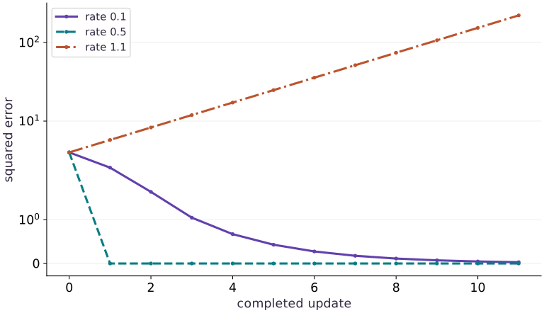
Gradient descent trades step size for stability

Predict before looking: Which rate will cause errors to grow rather than shrink?

Read the figure

The horizontal axis counts completed updates, including the initial state at $0$ . The vertical axis is squared error. It uses a symmetric-log scale: values near zero are on a linear region, while large values are compressed logarithmically. That lets the zero-loss trajectory remain visible.

All three curves begin at loss $4$ . Learning rate $0.1$ decreases it gradually; rate $0.5$ reaches zero after one update and stays there. Rate $1.1$ increases it from $4$ to $5.76$ , then beyond $200$ by the last plotted update.

Connect it to the computation

Here the loss is $(w-2)^2$ . One update multiplies the weight error $w-2$ by $1-2\eta$ . The three rates therefore multiply that error by $0.8$ , $0$ , and $-1.2$ , respectively. Squaring gives loss multipliers $0.64$ , $0$ , and $1.44$ .

The large rate crosses the optimum and lands farther away on each step. The loss plot shows the growing distance, while the sign change follows from the update equation; loss alone does not reveal which side the weight is on. The one-step success of rate $0.5$ depends on this simple quadratic’s curvature and is not a universal best learning rate.

Open full-size figure Download data and provenance

The notebook contains the data experiment, plotting code, and recorded figure output. Rerun it to test your changes.

Where to put & run this code: Work in phases/04-optimization/03-write-gradient-descent-yourself/code/main.py (or downloaded exercises/optimization-03.py / exercises/optimization-03.ipynb) and execute from the repository root with python3 phases/04-optimization/03-write-gradient-descent-yourself/code/main.py.

1 Prepare the inputs

Create a file named main.py in your activated learning environment. Add these imports and inputs first. Shapes and numeric types are part of the experiment.

main.py · append build step 1

# Step 1 — 1. Prepare the inputs: This block establishes the values used by the following steps; run...
import jax
import jax.numpy as jnp

This block establishes the values used by the following steps; run the completed file after step $3$ .

2 Define the computation

Append this block below the inputs. Before proceeding, trace which values are inputs, predictions, and state.

main.py · append build step 2

# Step 2 — 2. Define the computation: train defines a state transition that subtracts the derivative.
def loss(w):
    return (w - 2.) ** 2
# Define `train(initial, rate, steps)` to evaluate the objective and its automatic derivatives:
def train(initial, rate, steps):
    # Define `step(w, _)` to evaluate the objective and its automatic derivatives:
    def step(w, _):
        # Differentiate the objective to obtain `next_w` via automatic differentiation.
        next_w = w - rate * jax.grad(loss)(w)
        return next_w, loss(next_w)
    return jax.lax.scan(step, jnp.array(initial), None, length=steps)

Code building blocks in this step

jnp.array(values, dtype=...) — Constructs an immutable device-backed JAX array from Python/NumPy values.
jax.grad(loss_fn)(params, ...) — Transforms a scalar-output function into a function returning the gradient PyTree with the same structure as params.
jax.lax.scan(step_fn, init_carry, xs, length=...) — Compiles a sequential loop where step_fn(carry, x) returns (next_carry, y), returning (final_carry, stacked_ys).

train defines a state transition that subtracts the derivative. scan retains the new parameter and records its post-update loss for exactly steps iterations.

3 Measure and verify

Append the remaining block, then run python main.py in the terminal. Compare the printed result with the expected output below. Assertions stop execution if the contract fails.

main.py · append build step 3

# Step 3 — 3. Measure and verify: The weight approaches 2.0 and the final loss is below 10^{-8}.
final, history = train(0., 0.1, 60)
print("Final weight:", float(final))
print("Final loss:", float(history[-1]))
assert jnp.allclose(final, 2., atol=1e-4)
assert history[-1] < 1e-8
assert jnp.all(jnp.diff(history) <= 1e-7)

Code building blocks in this step

jnp.allclose(actual, expected, rtol=..., atol=...) — Checks that two arrays match elementwise within floating-point tolerance.

The weight approaches $2.0$ and the final loss is below $10^{-8}$ .

View the cumulative build in main.py

These blocks append in order to the same file.

main.py · cumulative Python build

# Step 1 — 1. Prepare the inputs: This block establishes the values used by the following steps; run...
import jax
import jax.numpy as jnp

# Step 2 — 2. Define the computation: train defines a state transition that subtracts the derivative.
def loss(w):
    return (w - 2.) ** 2
# Define `train(initial, rate, steps)` to evaluate the objective and its automatic derivatives:
def train(initial, rate, steps):
    # Define `step(w, _)` to evaluate the objective and its automatic derivatives:
    def step(w, _):
        # Differentiate the objective to obtain `next_w` via automatic differentiation.
        next_w = w - rate * jax.grad(loss)(w)
        return next_w, loss(next_w)
    return jax.lax.scan(step, jnp.array(initial), None, length=steps)

# Step 3 — 3. Measure and verify: The weight approaches 2.0 and the final loss is below 10^{-8}.
final, history = train(0., 0.1, 60)
print("Final weight:", float(final))
print("Final loss:", float(history[-1]))
assert jnp.allclose(final, 2., atol=1e-4)
assert history[-1] < 1e-8
assert jnp.all(jnp.diff(history) <= 1e-7)

Run the example

python3 phases/04-optimization/03-write-gradient-descent-yourself/code/main.py

About this command

This shortcut uses an activated macOS/Linux course environment in the repository folder. For Windows, use the explicit interpreter command in “Setup help” above. The script includes worked examples and reference solutions.

Inspect the complete assembled example

main.py · complete Python example

# Step 1 — 1. Prepare the inputs: This block establishes the values used by the following steps; run...
import jax
import jax.numpy as jnp
# Step 2 — 2. Define the computation: train defines a state transition that subtracts the derivative.
def loss(w):
    return (w - 2.) ** 2
# Define `train(initial, rate, steps)` to evaluate the objective and its automatic derivatives:
def train(initial, rate, steps):
    # Define `step(w, _)` to evaluate the objective and its automatic derivatives:
    def step(w, _):
        # Differentiate the objective to obtain `next_w` via automatic differentiation.
        next_w = w - rate * jax.grad(loss)(w)
        return next_w, loss(next_w)
    return jax.lax.scan(step, jnp.array(initial), None, length=steps)
# Step 3 — 3. Measure and verify: The weight approaches 2.0 and the final loss is below 10^{-8}.
final, history = train(0., 0.1, 60)
print("Final weight:", float(final))
print("Final loss:", float(history[-1]))
assert jnp.allclose(final, 2., atol=1e-4)
assert history[-1] < 1e-8
assert jnp.all(jnp.diff(history) <= 1e-7)

Expected result: The weight approaches $2.0$ and the final loss is below $10^{-8}$ .

Recorded reference execution

Reference output captured from executing the complete lesson script (code/main.py) and its assertions in the course CPU environment.

2026-10-20T10:45:48.289484+00:00 · Python 3.14.3 · JAX 0.9.2 · 1 CPU device

Final weight: 1.9999969005584717
Final loss: 9.606537787476555e-12
Final weight: 1.9999969005584717
Final loss: 9.606537787476555e-12
First two post-update losses: [2.5600002 1.6384   ]
PASS: optimization-03

Download execution record · The notebook includes executed cells and figure outputs. Compare your run with these values; timings depend on the machine.

Check the first two steps

Check the first two steps · Python experiment

# Experiment — Check the first two steps: A hand-derived trajectory checks update sign and the recording...
two_w, two_losses = train(0., 0.1, 2)
assert jnp.allclose(two_w, 0.72)
assert jnp.allclose(two_losses, jnp.array([2.56, 1.6384]))
print("First two post-update losses:", two_losses)

Expected: $[2.56, 1.6384]$ , with final weight $0.72$ .

A hand-derived trajectory checks update sign and the recording convention.

Test the edge of stability

Test the edge of stability · Python experiment

# Experiment — Test the edge of stability: Magnitude-one error multipliers do not contract even though the...
edge_w, edge_losses = train(0., 1., 5)
assert jnp.allclose(edge_w, 4.)
assert jnp.allclose(edge_losses, jnp.full(5, 4.))

Expected: The weight alternates $0$ and $4$ ; loss remains $4$ .

Magnitude-one error multipliers do not contract even though the loop remains finite.

A tiny update far from the solution

A tiny update far from the solution · Python experiment

# Experiment — A tiny update far from the solution: A stopping rule must distinguish lack of progress from reaching...
far = jnp.array(0.)
quadratic = lambda value: (value-2.)**2
# Differentiate the objective to obtain `grad_far` via automatic differentiation.
grad_far = jax.grad(quadratic)(far)
next_far = far - 1e-8*grad_far
assert jnp.abs(next_far-far)<1e-6
assert jnp.abs(grad_far)>3.
assert quadratic(next_far)>3.9

Expected: The update is below the threshold, but the objective is still near $4$ .

A stopping rule must distinguish lack of progress from reaching a useful solution.

Hands-On Exercise · Modify & Verify Run in the declared lesson environment

Make it yours

Where to put your code: Append your solution at the bottom of phases/04-optimization/03-write-gradient-descent-yourself/code/main.py (or inside the Make it yours cell of exercises/optimization-03.ipynb) and run python3 phases/04-optimization/03-write-gradient-descent-yourself/code/main.py to verify your prediction before opening the reference solution.

Run ten steps with learning rate $1.1$ . Predict whether the error contracts before executing; show evidence of divergence.

Show a writing guide and starter scaffold

How to write this exercise code: step-by-step recipe & starter scaffold

1. Key functions & syntax to use:

train(...) — Call train with your updated parameters or inputs from this lesson's workspace.
loss(...) — Call loss with your updated parameters or inputs from this lesson's workspace.
assert condition — Verify that the observed output shape, status, or numerical value satisfies the contract.

2. Step-by-step implementation plan:

Set up the changed input or configuration parameters requested in the prompt.
Run the target function or transformation and assert that the output matches your prediction.

Starter code scaffold · copy into your file & fill in the TODOs

# Exercise solution: Run ten steps with learning rate 1.1.
unstable, unstable_history = train(...)  # TODO: compute unstable, unstable_history
assert unstable_history[-1]  # TODO: complete assertion check
assert abs(1 - 2 * 1.1)  # TODO: complete assertion check

Reveal the reference solution

Reference solution

# Exercise solution: Run ten steps with learning rate 1.1.
unstable, unstable_history = train(0., 1.1, 10)
assert unstable_history[-1] > loss(0.)
assert abs(1 - 2 * 1.1) > 1

Transfer the stability analysis

Transfer / diagnosis

For $4(w-3)^2$ , derive a stable rate and verify convergence from zero.

Show a writing guide and starter scaffold

How to write this practice solution: step-by-step recipe & starter scaffold

1. Key functions & syntax to use:

jnp.array(values, dtype=...) — Constructs an immutable device-backed JAX array from Python/NumPy values.
jnp.allclose(actual, expected, rtol=..., atol=...) — Checks that two arrays match elementwise within floating-point tolerance.
jax.grad(loss_fn)(params, ...) — Transforms a scalar-output function into a function returning the gradient PyTree with the same structure as params.
jax.lax.scan(step_fn, init_carry, xs, length=...) — Compiles a sequential loop where step_fn(carry, x) returns (next_carry, y), returning (final_carry, stacked_ys).

2. Step-by-step implementation plan:

Define scaled_step(w, _) to evaluate the objective and its automatic derivatives:
Differentiate the objective to obtain new via automatic differentiation.
Run compiled structured control flow via jax.lax ((scaled_w, scaled_history)).

Starter code scaffold · copy into your file & fill in the TODOs

# Transfer the stability analysis (Transfer / diagnosis): Changing curvature changes the stability interval to...
def scaled_loss(w):
    return ...  # TODO: return computed result
# Define `scaled_step(w, _)` to evaluate the objective and its automatic derivatives:
def scaled_step(w, _):
    # Differentiate the objective to obtain `new` via automatic differentiation.
    new = ...  # TODO: compute new
    return ...  # TODO: return computed result
# Run compiled structured control flow via `jax.lax` (`(scaled_w, scaled_history)`).
scaled_w, scaled_history = jax.lax.scan(...)  # TODO: compute scaled_w, scaled_history
assert jnp.allclose(scaled_w, 3., atol=1e-5)  # TODO: complete assertion check
assert jnp.all(jnp.diff(scaled_history)  # TODO: complete assertion check

Show a hint

The error multiplier is $1-8\eta$ ; use $\eta=0.1$ .

Reveal reference solution and reasoning

Transfer the stability analysis · Python solution

# Transfer the stability analysis (Transfer / diagnosis): Changing curvature changes the stability interval to...
def scaled_loss(w):
    return 4*(w-3.)**2
# Define `scaled_step(w, _)` to evaluate the objective and its automatic derivatives:
def scaled_step(w, _):
    # Differentiate the objective to obtain `new` via automatic differentiation.
    new = w-0.1*jax.grad(scaled_loss)(w)
    return new, scaled_loss(new)
# Run compiled structured control flow via `jax.lax` (`(scaled_w, scaled_history)`).
scaled_w, scaled_history = jax.lax.scan(scaled_step, jnp.array(0.), None, length=20)
assert jnp.allclose(scaled_w, 3., atol=1e-5)
assert jnp.all(jnp.diff(scaled_history) <= 1e-6)

Changing curvature changes the stability interval to $0<\eta<0.25$ .

Reproduce an uphill update and repair it

Transfer / diagnosis

Show how adding the gradient increases loss, then verify subtraction at the same starting point.

Show a writing guide and starter scaffold

How to write this practice solution: step-by-step recipe & starter scaffold

1. Key functions & syntax to use:

jnp.allclose(actual, expected, rtol=..., atol=...) — Checks that two arrays match elementwise within floating-point tolerance.
jax.grad(loss_fn)(params, ...) — Transforms a scalar-output function into a function returning the gradient PyTree with the same structure as params.

2. Step-by-step implementation plan:

Differentiate the objective to obtain uphill via automatic differentiation.
Differentiate the objective to obtain downhill via automatic differentiation.

Starter code scaffold · copy into your file & fill in the TODOs

# Reproduce an uphill update and repair it (Transfer / diagnosis): The sign error is isolated using the same input and rate;...
# Differentiate the objective to obtain `uphill` via automatic differentiation.
uphill = ...  # TODO: compute uphill
# Differentiate the objective to obtain `downhill` via automatic differentiation.
downhill = ...  # TODO: compute downhill
assert loss(uphill)  # TODO: complete assertion check
assert loss(downhill)  # TODO: complete assertion check
assert jnp.allclose(downhill, 0.4)  # TODO: complete assertion check

Show a hint

The derivative at zero is $-4$ .

Reveal reference solution and reasoning

Reproduce an uphill update and repair it · Python solution

# Reproduce an uphill update and repair it (Transfer / diagnosis): The sign error is isolated using the same input and rate;...
# Differentiate the objective to obtain `uphill` via automatic differentiation.
uphill = 0. + 0.1*jax.grad(loss)(0.)
# Differentiate the objective to obtain `downhill` via automatic differentiation.
downhill = 0. - 0.1*jax.grad(loss)(0.)
assert loss(uphill) > loss(0.)
assert loss(downhill) < loss(0.)
assert jnp.allclose(downhill, 0.4)

The sign error is isolated using the same input and rate; the repaired first step matches the analytic result.

Diagnose the result

Record the loss trajectory and parameter values. An alternating, growing error here follows from the update equation; changing the PRNG seed cannot fix it.

Carry forward

A hand-derived trajectory checks update sign and the recording convention.
Magnitude-one error multipliers do not contract even though the loop remains finite.

Keep your evidence

Download evidence template

Keep the two hand-computed steps, rate stability derivation, edge/divergent runs, scaled-curvature transfer and uphill-update repair. Include the tiny-update counterexample and explain your stopping criteria.

Save your modified code, its output, and an explanation of your prediction. Checkpoint answers and exercise evidence are tracked separately.

Saved in this browser. Export or back up your portfolio anytime in My learning.

Save work for this lesson

Verified on local CPU. Stage to a Cloud TPU VM via Cloud TPU setup to record accelerator execution receipts (TODO: add automated Cloud TPU CI execution receipts).

Write gradient descent yourself

What you will be able to do

The problem

The idea

The sign tells you which way to step

Derive one update before writing the loop

Read the learning rate through curvature

Make the trajectory part of the state contract

Diagnose dynamics instead of only the final number

Use stopping evidence that survives rescaling

Gradient descent trades step size for stability

Read the figure

Connect it to the computation

1 Prepare the inputs

2 Define the computation

3 Measure and verify

Run the example

Recorded reference execution

Check the first two steps

Test the edge of stability

A tiny update far from the solution

Make it yours

Transfer the stability analysis

Reproduce an uphill update and repair it

Check your understanding

Diagnose the result

Carry forward

Keep your evidence

Primary references