 JAX Pathways
Phase 04 / Math & optimization
Minibatches, expectation, and gradient noise
Revision v0.7.0 · Updated since your last visit. Review the changes; your progress is saved.
Lesson · about 75 minutes · CPU practice
Explain an unbiased minibatch gradient and verify how sampling and reduction affect its variance.
Phase study guide: preparation, milestones and project evidence
Before you start
Before this: Regularization and honest validation
Hardware: CPU
Setup help: Python, notebook, or Cloud TPU VM
Use the tested CPU packages (the recorded environment uses Python 3.14.3). Other Python versions and accelerator environments require separate checks. The optional Cloud TPU specialization explains the target-specific execution boundaries. Logical CPU devices practice partitioning; they do not simulate TPU performance.
Download the repository ZIP or use your existing checkout. Extract it and open a terminal in the folder containing requirements-cpu.txt. The beginner ZIP is separate; these lessons use the full repository folder.
python3 -m venv .venv
source .venv/bin/activate
python -m pip install -r requirements-cpu.txtpy -3 -m venv .venv
.\.venv\Scripts\python.exe -m pip install -r requirements-cpu.txtAfter activation, run the complete worked example from that same folder:
python phases/04-optimization/11-minibatches-expectation-and-gradient-noise/code/main.py.\.venv\Scripts\python.exe phases/04-optimization/11-minibatches-expectation-and-gradient-noise/code/main.pyFor an incremental build, create main.py in your own practice folder, append each build block in order, and run python main.py with this environment active. Keep that file separate from the downloaded reference solution.
Download this lesson’s notebook. Open it with a Python kernel using the course environment. Run cells from the top after restarting the kernel; experiments depend on earlier definitions.
For local Jupyter, first install the course requirements using the Local Python steps, then use your environment’s Python to start Jupyter:
python -m pip install jupyterlab
python -m jupyter lab.\.venv\Scripts\python.exe -m pip install jupyterlab
.\.venv\Scripts\python.exe -m jupyter labSelect the downloaded optimization-11.ipynb file in JupyterLab. The notebook contains reference solutions; make your prediction and attempt each practice task before opening them. Restart the kernel before changing logical device setup.
The worked reference for this lesson is CPU-validated. Some references explicitly configure logical CPU devices; setting JAX_PLATFORMS does not adapt them to a TPU. Follow the execution matrix and reviewed multi-host example before attempting a target run.
For accelerator preparation, study TPU setup, observed runtime receipts, checkpointed jobs and precision and retained traces. These target paths remain unqualified on physical TPU hardware until an actual receipt is recorded. Cloud provisioning is optional for CPU learning.
Check: Full gradient ; variances for one example and for two independent draws.
Revisit the guided CPU setup · Open 19: TPU Setup. Package instructions are CPU instructions; Windows and accelerator environments need their own validation.
What you will be able to do
- Explain an unbiased minibatch gradient and verify how sampling and reduction affect its variance.
- Define the population before estimating it
- Make the independence assumption explicit
- Weight unequal batches by example count
- Separate noise, replay and progress
The problem
A minibatch may suggest a different update from the full dataset. Is it wrong, or is it a noisy estimate? We will enumerate every possible tiny batch so expectation and variance become quantities you can inspect rather than claims you have to trust.
The idea
A minibatch gradient estimates the full-data gradient using fewer examples. Its noise depends on the sampling scheme and batch size. When combining batches, the denominator must still represent the population you intend to average over.
Average examples rather than batch averages
Suppose one batch has two examples with mean loss , and another has one example with loss . Averaging batch means gives . The mean over all three examples is . The first calculation gave the small batch too much weight.
Carry loss sums and example counts through aggregation, then divide once. For token losses, carry valid-token counts instead: examples and tokens are different denominators when lengths vary. The same weighting issue appears when combining gradients across devices.
The variance plot illustrates the benefit of averaging under its stated sampling assumptions. Correlated examples, sampling without replacement, and nonuniform sampling can change the relationship. Batch size alone does not fully describe the estimator.
Define the population before estimating it
Use the per-example loss with targets . At , the per-example gradients are . Their mean is , and their population variance is : average the squared deviations from the mean, dividing by . This finite training dataset is the population for our sampling experiment, not the population of all future data.
Make the independence assumption explicit
Draw examples independently and uniformly with replacement, where is the batch size. Repeated examples are allowed. The batch gradient has expectation and variance . For , enumerate all ordered pairs. The batch variance is . Sampling without replacement follows a different variance formula; correlated samples can reduce the benefit of averaging.
Weight unequal batches by example count
A batch mean over three examples and a batch mean over one example should not receive equal weight when reconstructing the dataset mean. Our first three gradients average to , while the last is . Averaging those means gives , which is wrong. Weighting by counts gives . The same issue appears when accumulating gradients or aggregating metrics across devices.
Separate noise, replay and progress
A random key records a reproducible sampling choice; reusing it repeats that choice. Split keys for fresh batches. An individual minibatch update can worsen the full loss even though its gradient is unbiased at the current parameters. Log full or held-out evaluation at defined intervals instead of expecting a monotone minibatch curve. Unbiasedness alone does not prove convergence, and changing batch size can change both compute cost and optimization behavior.
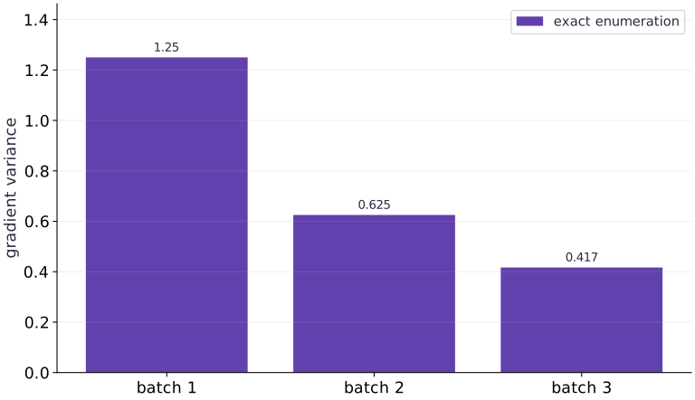
Averaging independent gradients reduces variance
Predict before looking: How much variance remains when the batch grows from to ?
Read the figure
The horizontal categories are batch sizes , , and . The vertical axis is the variance of the estimated gradient at one fixed weight. The bar heights are , , and approximately , respectively.
Doubling the batch size from to halves the variance. Tripling it divides the variance by . These are exact enumerations of the possible sampled batches in this small example, rather than noisy estimates from a handful of trials.
Connect it to the computation
Each batch averages independent, uniformly sampled per-example gradients with replacement. Under those assumptions, the variance of the average is the single-example variance divided by batch size. Its expected gradient remains for all three sizes; the estimate becomes less variable without changing its mean.
The bar heights are squared gradient units, not loss or gradient magnitude. A shorter bar does not mean a smaller learning rate or a faster overall training run. Sampling without replacement, correlated examples, and changing parameters require a different variance analysis.
Open full-size figureDownload data and provenance
The notebook contains the data experiment, plotting code, and recorded figure output. Rerun it to test your changes.
Where to put & run this code: Work in phases/04-optimization/11-minibatches-expectation-and-gradient-noise/code/main.py (or downloaded exercises/optimization-11.py / exercises/optimization-11.ipynb) and execute from the repository root with python3 phases/04-optimization/11-minibatches-expectation-and-gradient-noise/code/main.py.
1 Compute per-example gradients
Create main.py. Keep the parameter fixed while measuring the sampling distribution.
# Step 1 — Compute per-example gradients: Each example supplies a slope; the dataset objective uses their mean.
import jax
import jax.numpy as jnp
y = jnp.array([1.0, 2.0, 3.0, 4.0])
w = jnp.array(0.0)

def example_loss(w, y):
    return 0.5 * (w - y) ** 2
# Differentiate the objective to obtain `per` via automatic differentiation.
per = jax.vmap(jax.grad(example_loss), in_axes=(None, 0))(w, y)
# Differentiate the objective to obtain `full` via automatic differentiation.
full = jax.grad(lambda w: jnp.mean(jax.vmap(example_loss, in_axes=(None, 0))(w, y)))(w)
assert jnp.allclose(per, jnp.array([-1.0, -2.0, -3.0, -4.0]))
assert jnp.allclose(full, -2.5)
Code building blocks in this step
jnp.array(values, dtype=...)— Constructs an immutable device-backed JAX array from Python/NumPy values.x.sum(axis=...) / x.mean(axis=..., keepdims=...)— Reduces values along the namedaxis(the axis you name is collapsed unlesskeepdims=True).jnp.allclose(actual, expected, rtol=..., atol=...)— Checks that two arrays match elementwise within floating-point tolerance.jax.grad(loss_fn)(params, ...)— Transforms a scalar-output function into a function returning the gradient PyTree with the same structure asparams.
Each example supplies a slope; the dataset objective uses their mean.
2 Enumerate every pair
Append the exact with-replacement distribution. No random simulation is needed for this check.
# Step 2 — Enumerate every pair: All ordered pairs are equally likely under independent uniform draws.
pairs = (per[:, None] + per[None, :]) / 2
# Check tensor shape invariant: `pairs.shape == (4, 4)`
assert pairs.shape == (4, 4)
assert jnp.allclose(jnp.mean(pairs), full)
assert jnp.allclose(jnp.var(per), 1.25)
assert jnp.allclose(jnp.var(pairs), 0.625)
Code building blocks in this step
x.sum(axis=...) / x.mean(axis=..., keepdims=...)— Reduces values along the namedaxis(the axis you name is collapsed unlesskeepdims=True).jnp.allclose(actual, expected, rtol=..., atol=...)— Checks that two arrays match elementwise within floating-point tolerance.
All ordered pairs are equally likely under independent uniform draws.
3 Sample and replay one batch
Append a PRNG example and run python main.py.
# Step 3 — Sample and replay one batch: Replay checks reproducibility.
# Create or split explicit PRNG key(s) (`key`) for reproducible randomness.
key = jax.random.key(7)
# Sample deterministic random values into `indices` using an explicit PRNG key.
indices = jax.random.choice(key, 4, shape=(2,), replace=True)
# Sample deterministic random values into `replay` using an explicit PRNG key.
replay = jax.random.choice(key, 4, shape=(2,), replace=True)
assert jnp.array_equal(indices, replay)
print('full gradient / single variance / pair variance:', full, jnp.var(per), jnp.var(pairs))
print('sample indices / sample gradient:', indices, jnp.mean(per[indices]))
Code building blocks in this step
x.sum(axis=...) / x.mean(axis=..., keepdims=...)— Reduces values along the namedaxis(the axis you name is collapsed unlesskeepdims=True).jax.random.PRNGKey(seed) & jax.random.split(key)— Manages explicit, stateless PRNG keys—always split a key before passing subkeys into independent random draws.
Replay checks reproducibility. One sample does not estimate the full sampling distribution.
View the cumulative build in main.py
These blocks append in order to the same file.
# Step 1 — Compute per-example gradients: Each example supplies a slope; the dataset objective uses their mean.
import jax
import jax.numpy as jnp
y = jnp.array([1.0, 2.0, 3.0, 4.0])
w = jnp.array(0.0)

def example_loss(w, y):
    return 0.5 * (w - y) ** 2
# Differentiate the objective to obtain `per` via automatic differentiation.
per = jax.vmap(jax.grad(example_loss), in_axes=(None, 0))(w, y)
# Differentiate the objective to obtain `full` via automatic differentiation.
full = jax.grad(lambda w: jnp.mean(jax.vmap(example_loss, in_axes=(None, 0))(w, y)))(w)
assert jnp.allclose(per, jnp.array([-1.0, -2.0, -3.0, -4.0]))
assert jnp.allclose(full, -2.5)

# Step 2 — Enumerate every pair: All ordered pairs are equally likely under independent uniform draws.
pairs = (per[:, None] + per[None, :]) / 2
# Check tensor shape invariant: `pairs.shape == (4, 4)`
assert pairs.shape == (4, 4)
assert jnp.allclose(jnp.mean(pairs), full)
assert jnp.allclose(jnp.var(per), 1.25)
assert jnp.allclose(jnp.var(pairs), 0.625)

# Step 3 — Sample and replay one batch: Replay checks reproducibility.
# Create or split explicit PRNG key(s) (`key`) for reproducible randomness.
key = jax.random.key(7)
# Sample deterministic random values into `indices` using an explicit PRNG key.
indices = jax.random.choice(key, 4, shape=(2,), replace=True)
# Sample deterministic random values into `replay` using an explicit PRNG key.
replay = jax.random.choice(key, 4, shape=(2,), replace=True)
assert jnp.array_equal(indices, replay)
print('full gradient / single variance / pair variance:', full, jnp.var(per), jnp.var(pairs))
print('sample indices / sample gradient:', indices, jnp.mean(per[indices]))
Run the example
python3 phases/04-optimization/11-minibatches-expectation-and-gradient-noise/code/main.pyAbout this command
This shortcut uses an activated macOS/Linux course environment in the repository folder. For Windows, use the explicit interpreter command in “Setup help” above. The script includes worked examples and reference solutions.
Inspect the complete assembled example
# Step 1 — Compute per-example gradients: Each example supplies a slope; the dataset objective uses their mean.
import jax
import jax.numpy as jnp
y = jnp.array([1.0, 2.0, 3.0, 4.0])
w = jnp.array(0.0)

def example_loss(w, y):
    return 0.5 * (w - y) ** 2
# Differentiate the objective to obtain `per` via automatic differentiation.
per = jax.vmap(jax.grad(example_loss), in_axes=(None, 0))(w, y)
# Differentiate the objective to obtain `full` via automatic differentiation.
full = jax.grad(lambda w: jnp.mean(jax.vmap(example_loss, in_axes=(None, 0))(w, y)))(w)
assert jnp.allclose(per, jnp.array([-1.0, -2.0, -3.0, -4.0]))
assert jnp.allclose(full, -2.5)

# Step 2 — Enumerate every pair: All ordered pairs are equally likely under independent uniform draws.
pairs = (per[:, None] + per[None, :]) / 2
# Check tensor shape invariant: `pairs.shape == (4, 4)`
assert pairs.shape == (4, 4)
assert jnp.allclose(jnp.mean(pairs), full)
assert jnp.allclose(jnp.var(per), 1.25)
assert jnp.allclose(jnp.var(pairs), 0.625)

# Step 3 — Sample and replay one batch: Replay checks reproducibility.
# Create or split explicit PRNG key(s) (`key`) for reproducible randomness.
key = jax.random.key(7)
# Sample deterministic random values into `indices` using an explicit PRNG key.
indices = jax.random.choice(key, 4, shape=(2,), replace=True)
# Sample deterministic random values into `replay` using an explicit PRNG key.
replay = jax.random.choice(key, 4, shape=(2,), replace=True)
assert jnp.array_equal(indices, replay)
print('full gradient / single variance / pair variance:', full, jnp.var(per), jnp.var(pairs))
print('sample indices / sample gradient:', indices, jnp.mean(per[indices]))
Expected result: Full gradient ; variances for one example and for two independent draws.
Recorded reference execution
Reference output captured from executing the complete lesson script (code/main.py) and its assertions in the course CPU environment.
full gradient / single variance / pair variance: -2.5 1.25 0.625
sample indices / sample gradient: [3 2] -3.5
full gradient / single variance / pair variance: -2.5 1.25 0.625
sample indices / sample gradient: [3 2] -3.5
PASS: optimization-11
Download execution record · The notebook includes executed cells and figure outputs. Compare your run with these values; timings depend on the machine.
Combine unequal batches
# Experiment — Combine unequal batches: Batch means require example-count weights when batch sizes differ.
# Aggregate array values to compute `first`.
first = jnp.mean(per[:3])
# Aggregate array values to compute `last`.
last = jnp.mean(per[3:])
wrong = (first + last) / 2
correct = (3 * first + last) / 4
assert jnp.allclose(wrong, -3.0)
assert jnp.allclose(correct, full)
Expected: The unweighted result is , while count weighting recovers .
Batch means require example-count weights when batch sizes differ.
Take a noisy step at the full optimum
# Experiment — Take a noisy step at the full optimum: A noisy gradient may point away from the full optimum on a...
# Aggregate array values to compute `full_loss`.
full_loss = lambda w: jnp.mean(0.5 * (w - y) ** 2)
optimum = jnp.array(2.5)
# Differentiate the objective to obtain `noisy` via automatic differentiation.
noisy = optimum - 0.1 * jax.grad(example_loss)(optimum, y[0])
assert jnp.allclose(jax.grad(full_loss)(optimum), 0.0)
assert full_loss(noisy) > full_loss(optimum)
Expected: The single-example step increases the full-data loss.
A noisy gradient may point away from the full optimum on a particular draw.
Make it yours
Where to put your code: Append your solution at the bottom of phases/04-optimization/11-minibatches-expectation-and-gradient-noise/code/main.py (or inside the Make it yours cell of exercises/optimization-11.ipynb) and run python3 phases/04-optimization/11-minibatches-expectation-and-gradient-noise/code/main.py to verify your prediction before opening the reference solution.
Enumerate all ordered batches of size . Check their mean and variance against the independent-sampling formula.
Show a writing guide and starter scaffold
How to write this exercise code: step-by-step recipe & starter scaffold
1. Key functions & syntax to use:
x.sum(axis=...) / x.mean(axis=..., keepdims=...)— Reduces values along the namedaxis(the axis you name is collapsed unlesskeepdims=True).jnp.allclose(actual, expected, rtol=..., atol=...)— Checks that two arrays match elementwise within floating-point tolerance.
2. Step-by-step implementation plan:
- Set up the changed input or configuration parameters requested in the prompt.
- Run the target function or transformation and assert that the output matches your prediction.
# Exercise solution: Enumerate all 64 ordered batches of size 3.
triples = ...  # TODO: compute triples
assert triples.size  # TODO: complete assertion check
assert jnp.allclose(jnp.mean(triples), full, atol=1e-06)  # TODO: complete assertion check
assert jnp.allclose(jnp.var(triples), 1.25 / 3, atol=1e-06)  # TODO: complete assertion check
Reveal the reference solution
# Exercise solution: Enumerate all 64 ordered batches of size 3.
triples = (per[:, None, None] + per[None, :, None] + per[None, None, :]) / 3
assert triples.size == 64
assert jnp.allclose(jnp.mean(triples), full, atol=1e-06)
assert jnp.allclose(jnp.var(triples), 1.25 / 3, atol=1e-06)
Accumulate before updating
Transfer / diagnosis
At the same fixed , accumulate gradients from microbatches of sizes and . Verify that one update matches the full-batch update.
Show a writing guide and starter scaffold
How to write this practice solution: step-by-step recipe & starter scaffold
1. Key functions & syntax to use:
x.sum(axis=...) / x.mean(axis=..., keepdims=...)— Reduces values along the namedaxis(the axis you name is collapsed unlesskeepdims=True).jnp.allclose(actual, expected, rtol=..., atol=...)— Checks that two arrays match elementwise within floating-point tolerance.jax.grad(loss_fn)(params, ...)— Transforms a scalar-output function into a function returning the gradient PyTree with the same structure asparams.
2. Step-by-step implementation plan:
- Differentiate the objective to obtain
g1via automatic differentiation. - Differentiate the objective to obtain
g2via automatic differentiation.
# Accumulate before updating (Transfer / diagnosis): Exact accumulation matches the full mean gradient only when...
# Differentiate the objective to obtain `g1` via automatic differentiation.
g1 = jax.grad(...)  # TODO: compute g1
# Differentiate the objective to obtain `g2` via automatic differentiation.
g2 = jax.grad(...)  # TODO: compute g2
accumulated = ...  # TODO: compute accumulated
assert jnp.allclose(w - 0.1 * accumulated, w - 0.1 * full)  # TODO: complete assertion check
Show a hint
Do not update parameters between microbatches. Weight each mean by its sample count.
Reveal reference solution and reasoning
# Accumulate before updating (Transfer / diagnosis): Exact accumulation matches the full mean gradient only when...
# Differentiate the objective to obtain `g1` via automatic differentiation.
g1 = jax.grad(lambda z: jnp.mean(0.5 * (z - y[:3]) ** 2))(w)
# Differentiate the objective to obtain `g2` via automatic differentiation.
g2 = jax.grad(lambda z: jnp.mean(0.5 * (z - y[3:]) ** 2))(w)
accumulated = (3 * g1 + g2) / 4
assert jnp.allclose(w - 0.1 * accumulated, w - 0.1 * full)
Exact accumulation matches the full mean gradient only when all microbatches use the same parameters and the reduction is correct.
Detect a biased sampler
Transfer / diagnosis
A sampler chooses targets and with probabilities and , never the others. Compute its expected gradient. Does it estimate the uniform dataset gradient?
Show a writing guide and starter scaffold
How to write this practice solution: step-by-step recipe & starter scaffold
1. Key functions & syntax to use:
jnp.allclose(actual, expected, rtol=..., atol=...)— Checks that two arrays match elementwise within floating-point tolerance.
2. Step-by-step implementation plan:
- Set up the changed input or configuration parameters requested in the prompt.
- Run the target function or transformation and assert that the output matches your prediction.
# Detect a biased sampler (Transfer / diagnosis): Uniform mean-gradient claims require the corresponding...
biased = ...  # TODO: compute biased
assert jnp.allclose(biased, -1.3)  # TODO: complete assertion check
assert not jnp.allclose(biased, full)  # TODO: complete assertion check
Show a hint
Use the sampling probabilities as weights. Missing examples cannot be recovered by naive averaging.
Reveal reference solution and reasoning
# Detect a biased sampler (Transfer / diagnosis): Uniform mean-gradient claims require the corresponding...
biased = 0.9 * per[0] + 0.1 * per[3]
assert jnp.allclose(biased, -1.3)
assert not jnp.allclose(biased, full)
Uniform mean-gradient claims require the corresponding sampling assumptions. A biased sampler changes the expected objective unless properly corrected.
Diagnose the result
If changing batch size unexpectedly scales the gradient, inspect sum versus mean and accumulation weights. If replay fails, retain the key and sampled indices. If the estimate stays biased over many draws, inspect the sampling distribution rather than only increasing batch size.
Carry forward
- Batch means require example-count weights when batch sizes differ.
- A noisy gradient may point away from the full optimum on a particular draw.
Keep your evidence
Keep the exact per-example mean, enumerated batch-variance calculation, uneven-batch repair, PRNG replay and gradient-accumulation check.
Save your modified code, its output, and an explanation of your prediction. Checkpoint answers and exercise evidence are tracked separately.
Saved in this browser. Export or back up your portfolio anytime in My learning.
Verified on local CPU. Stage to a Cloud TPU VM via Cloud TPU setup to record accelerator execution receipts (TODO: add automated Cloud TPU CI execution receipts).